Indel Diversity
Reading Config File:
knitr::opts_chunk$set(echo = TRUE, warning = FALSE, message = FALSE)
suppressMessages(suppressWarnings(library(knitr)))
suppressMessages(suppressWarnings(library(ggplot2)))
suppressMessages(suppressWarnings(library(ggrepel)))
suppressMessages(suppressWarnings(library(data.table)))
suppressMessages(suppressWarnings(library(rtracklayer)))
suppressMessages(suppressWarnings(library(plotly)))
suppressMessages(suppressWarnings(library(GenomicRanges)))
suppressMessages(suppressWarnings(library(parallel)))
suppressMessages(suppressWarnings(library(pbapply)))
suppressMessages(suppressWarnings(library(DT)))

targetName <- params$target_name
config <- yaml::read_yaml('./config.yml')
sampleSheet <- data.table::fread(config$sample_sheet)
pipeline_output_dir <- config$pipeline_output_dir
cut_sites <- rtracklayer::import.bed(config$cut_sites_file)
sampleComparisons <- data.table::fread(config$comparisons_file)
Declare some common functions
importSampleBigWig <- function(pipeline_output_dir, samples, suffix = '.alnCoverage.bigwig') {
  sapply(simplify = F, USE.NAMES = T,
                      X = unique(as.character(samples)),
                      FUN = function(s) {
  f <- file.path(pipeline_output_dir, 'indels', s, paste0(s, suffix))
  if(file.exists(f)) {
    rtracklayer::import.bw(f, as = 'RleList')
  } else {
    stop("Can't find bigwig file for sample: ",s," at: ",
         "\n",f,"\n")
  }})
}

subsetRleListByRange <- function(input.rle, input.gr) {
  as.vector(input.rle[[seqnames(input.gr)]])[start(input.gr):end(input.gr)]
}


getReadsWithIndels <- function(pipeline_output_dir, samples) {
  readsWithIndels <- lapply(samples, function(sample) {
  dt <- data.table::fread(file.path(pipeline_output_dir,
                                                 'indels',
                                                 sample,
                                                 paste0(sample, ".reads_with_indels.tsv")))
  })
  names(readsWithIndels) <- samples
  return(readsWithIndels)
}

getIndels <- function(pipeline_output_dir, samples) {
  indels <- sapply(simplify = FALSE, samples, function(s) {
  f <- file.path(pipeline_output_dir,
                 'indels',
                 s,
                 paste0(s, ".indels.tsv"))
  if(file.exists(f)) {
    dt <- data.table::fread(f)
    dt$sample <- s
    return(dt)
  } else {
    stop("Can't open indels.tsv file for sample",s,
            "at",f,"\n")
  }})
  return(indels)
}
Subset sample sheet for those that match the target region of interest
targetName <- params$target_name
sampleSheet <- sampleSheet[target_name == targetName]
targetRegion <- as(sampleSheet[target_name == targetName]$target_region[1], 'GRanges')

#get the list of all guides used for the target region
#get sample-specific cut sites at the target region
sgRNAs <- unlist(strsplit(x = sampleSheet[sampleSheet$target_name == targetName,]$sgRNA_ids,
                   split = ':'))
cutSites <- cut_sites[cut_sites$name %in% sgRNAs]
#import deletion coordinates
deletions <- do.call(rbind, lapply(getIndels(pipeline_output_dir, sampleSheet$sample_name),
function(dt) {
dt[indelType == 'D']
}))
sampleGuides <- lapply(sampleSheet$sample_name, function(s) {
sgRNAs <- unlist(strsplit(x = sampleSheet[sampleSheet$sample_name == s,]$sgRNA_ids,
split = ':'))
if(sgRNAs[1] == 'none') {
sgRNAs <- setdiff(unique(unlist(strsplit(x = sampleSheet[target_name == targetName,]$sgRNA_ids, split = ':'))), 'none')
}
return(sgRNAs)
})
names(sampleGuides) <- as.character(sampleSheet$sample_name)#find cut sites overlapping with the indels
# indels: a data.table object with minimal columns: start, end,
# cutSites: a GRanges object of cut site coordinates
# return: data.frame (nrow = nrow(indels), columns are sgRNA ids,
# values are 1 if indel overlaps cutsite, otherwise 0.
overlapCutSites <- function(indels, cutSites, extend = 5) {
cutSites_ext <- flank(cutSites, width = extend, both = TRUE)
#check if indel overlaps with the cut site
query <- GenomicRanges::makeGRangesFromDataFrame(indels)
overlaps <- as.data.table(findOverlaps(query, cutSites_ext, type = 'any', ignore.strand = TRUE))
M <- matrix(data = rep(0, nrow(indels) * length(cutSites)),
nrow = nrow(indels), ncol = length(cutSites))
colnames(M) <- cutSites$name
M[as.matrix(overlaps)] <- 1
return(M)
}
#get deletions within the target region
deletions <- as.data.table(subsetByOverlaps(GRanges(deletions), targetRegion, ignore.strand = TRUE))
#define deletion frequency: read support / coverage
deletions$freq <- deletions$ReadSupport/deletions$coverage
#find overlaps with cut sites (only considering guides used in the corresponding sample)
deletionCutsiteOverlaps <- cbind(deletions, overlapCutSites(deletions, cutSites))
deletionCutsiteOverlaps <- do.call(rbind, lapply(unique(deletionCutsiteOverlaps$sample), function(sampleName) {
dt <- deletionCutsiteOverlaps[sample == sampleName]
sgRNAs <- sampleGuides[[sampleName]]
dt$atCutSite <- apply(subset(dt, select = sgRNAs), 1, function(x) sum(x > 0) > 0)
return(dt)
}))# cs: data.frame with cut site coordinates. minimual columns: start, end, name
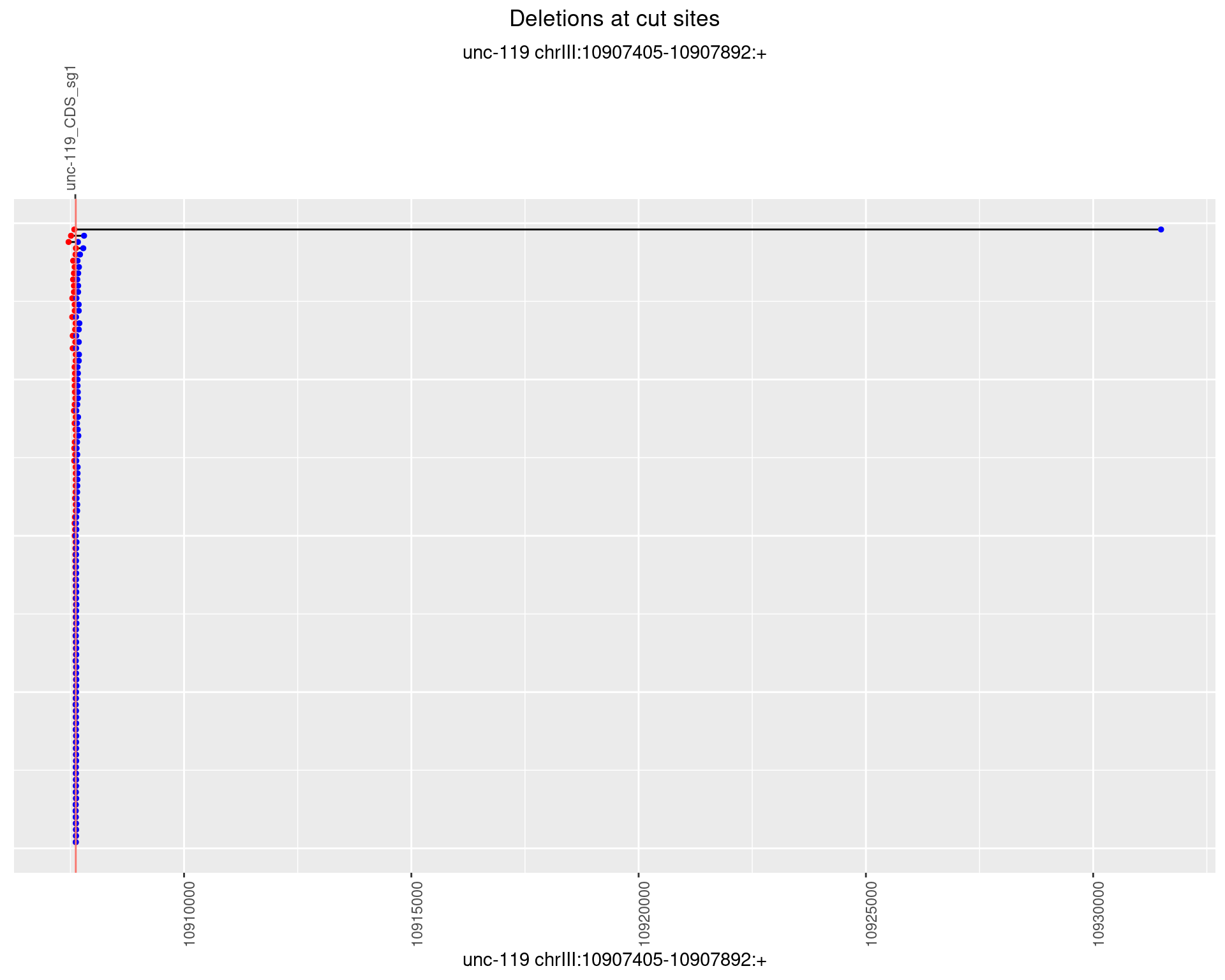
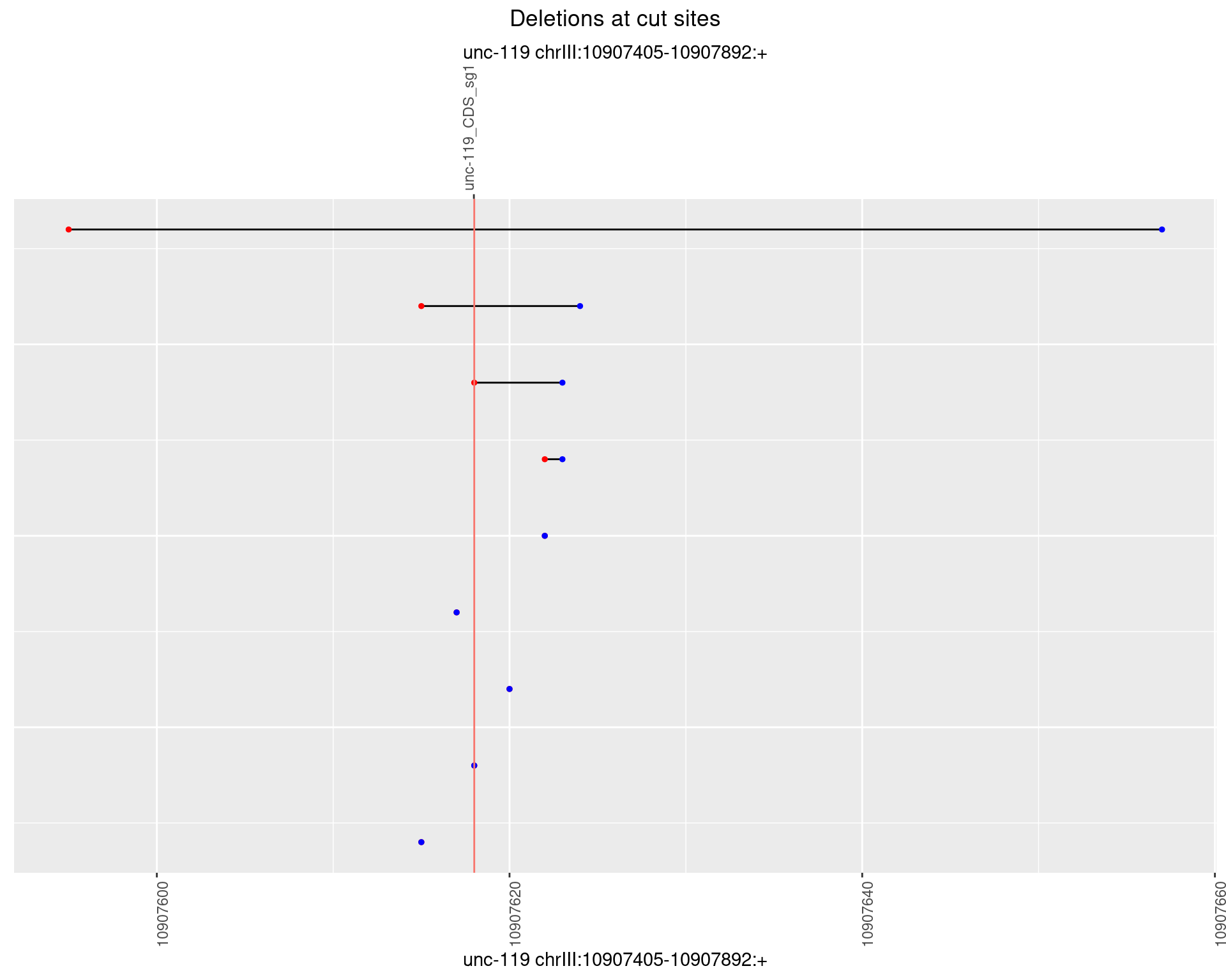
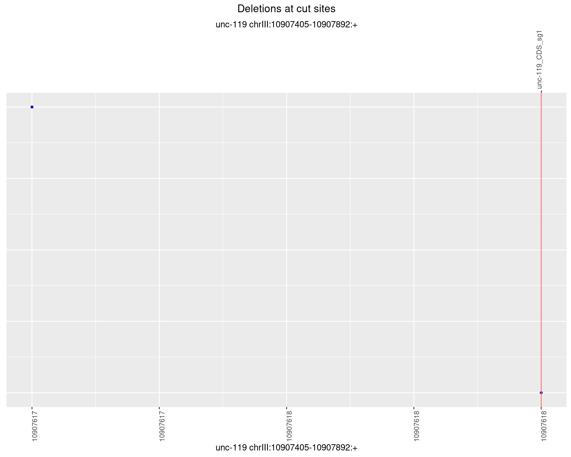
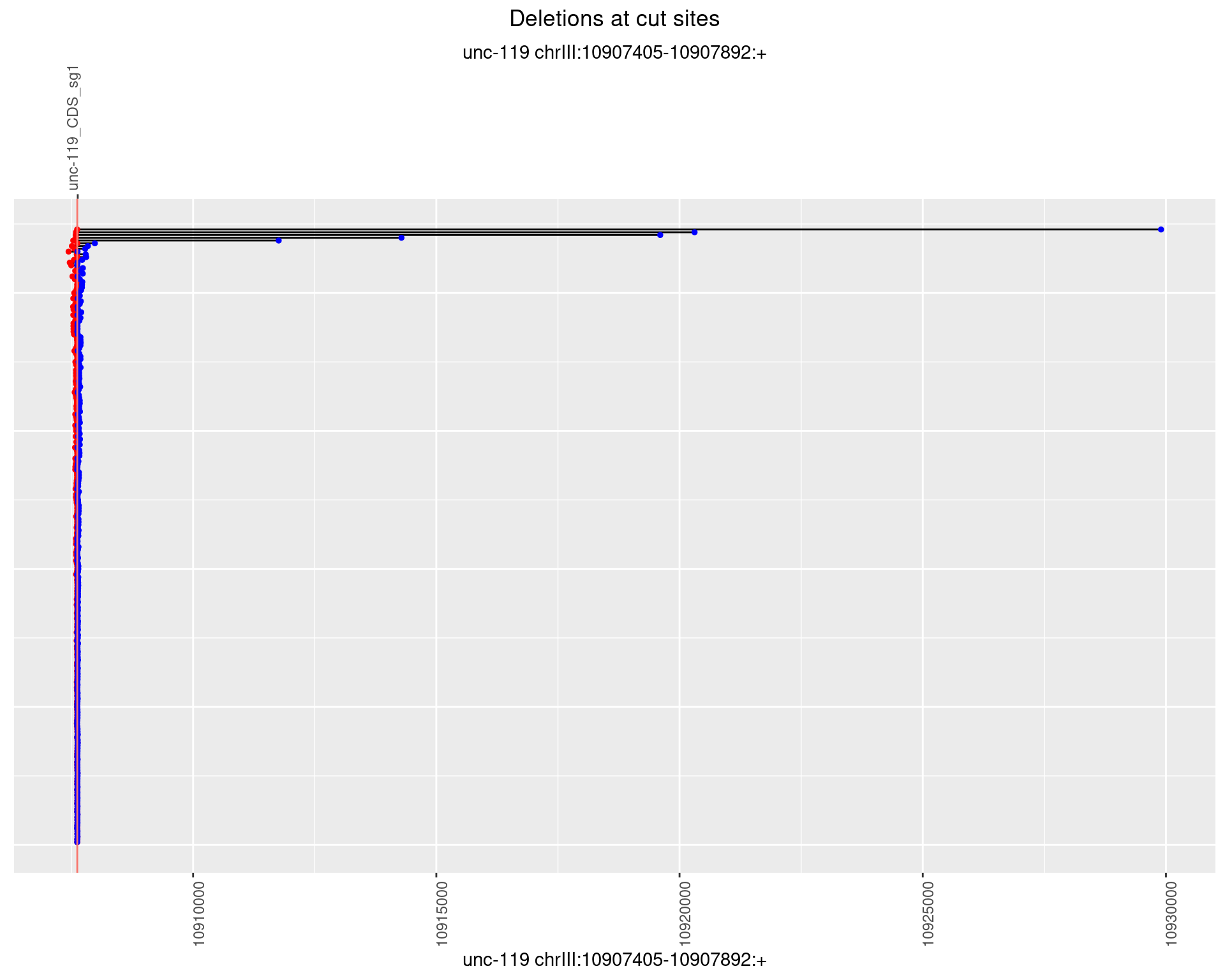
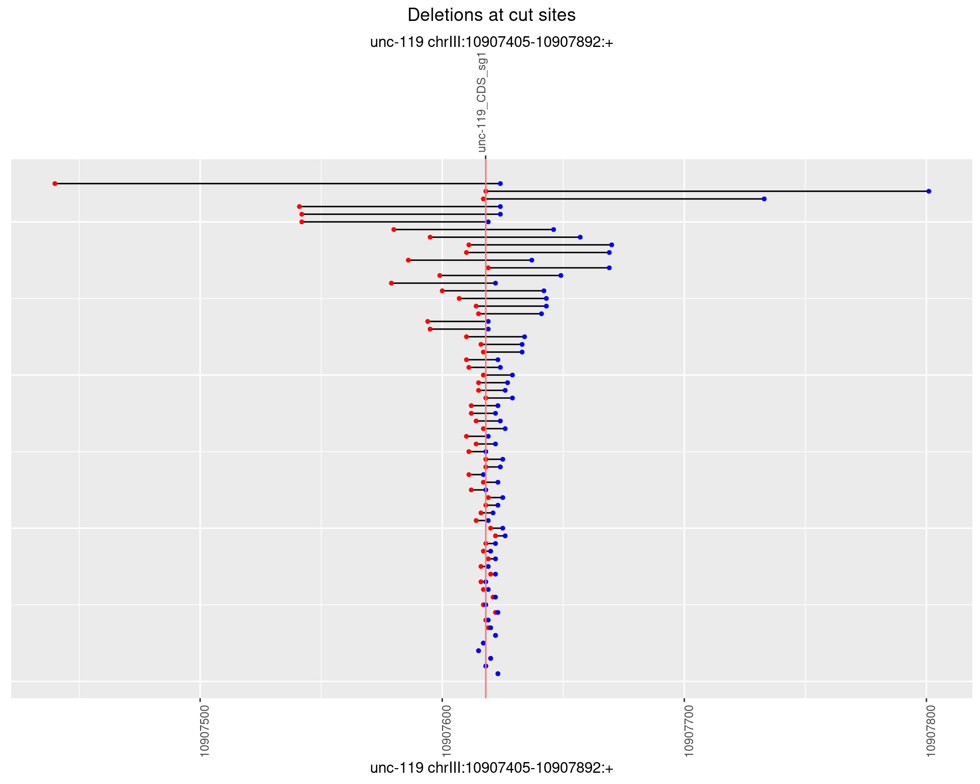
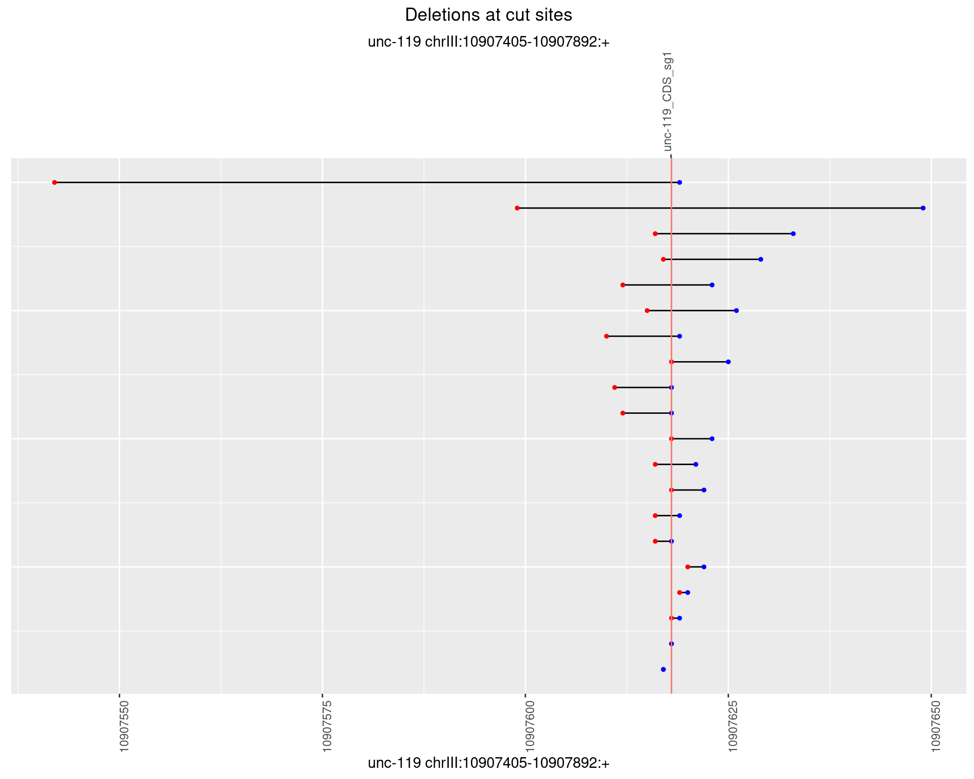
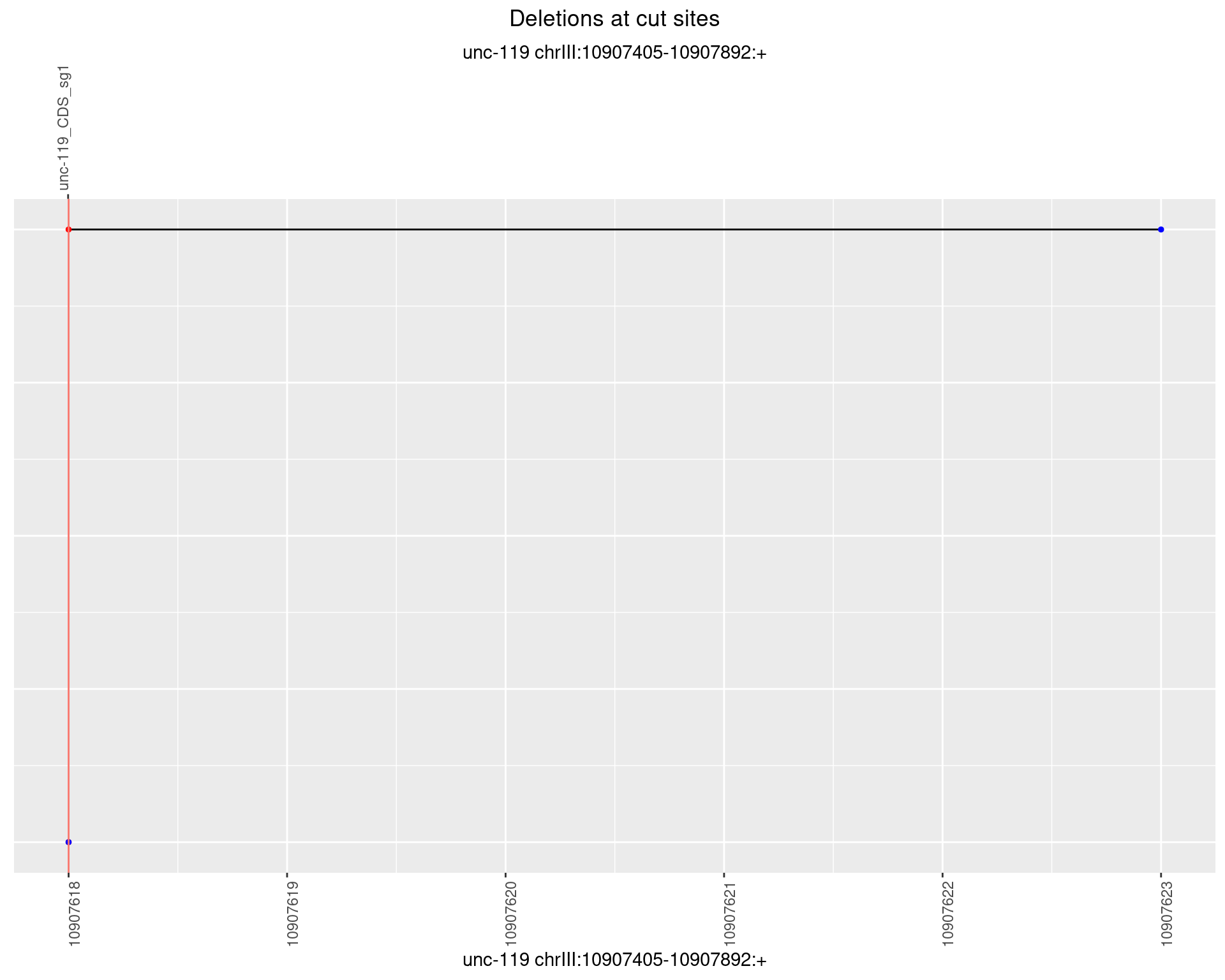
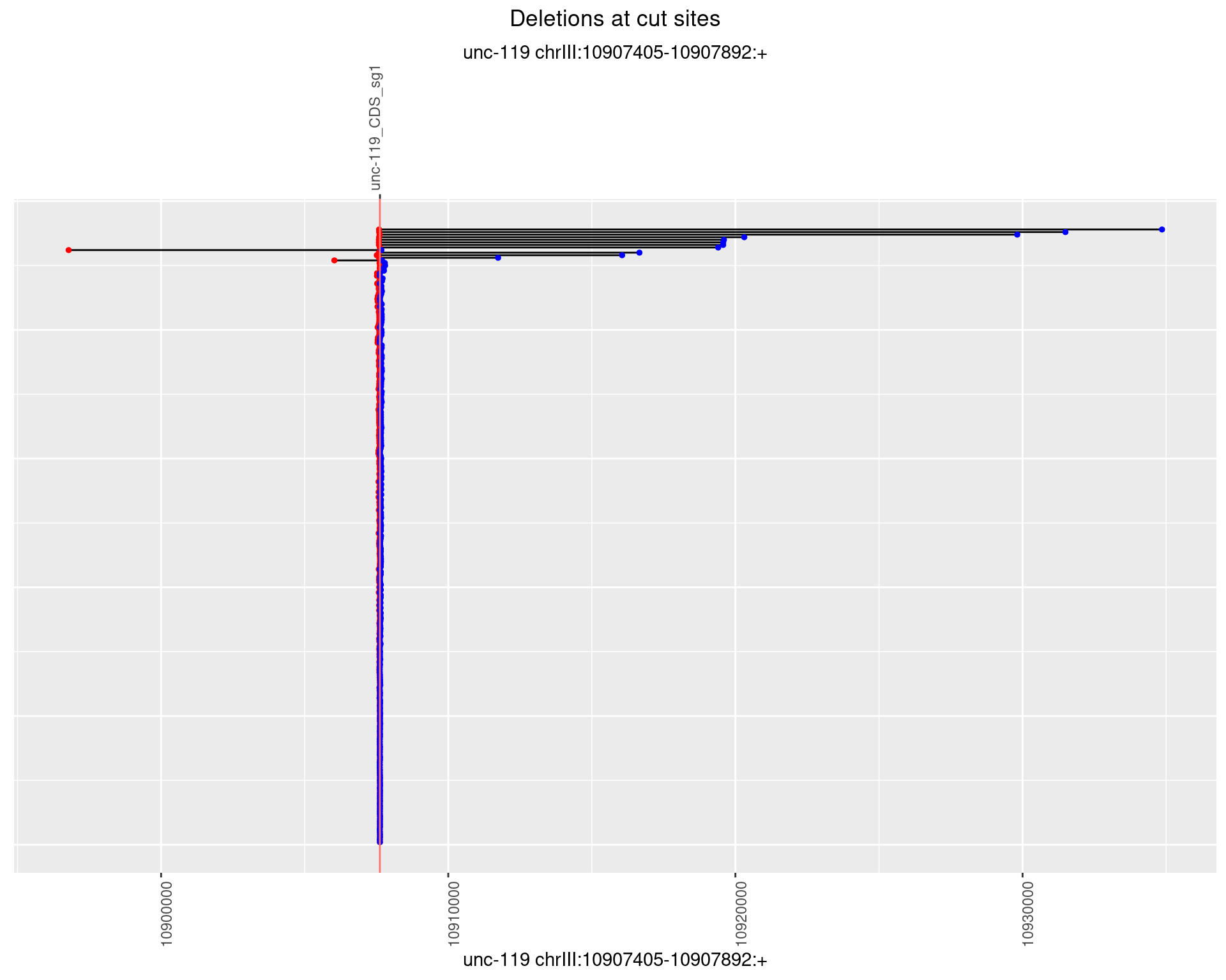
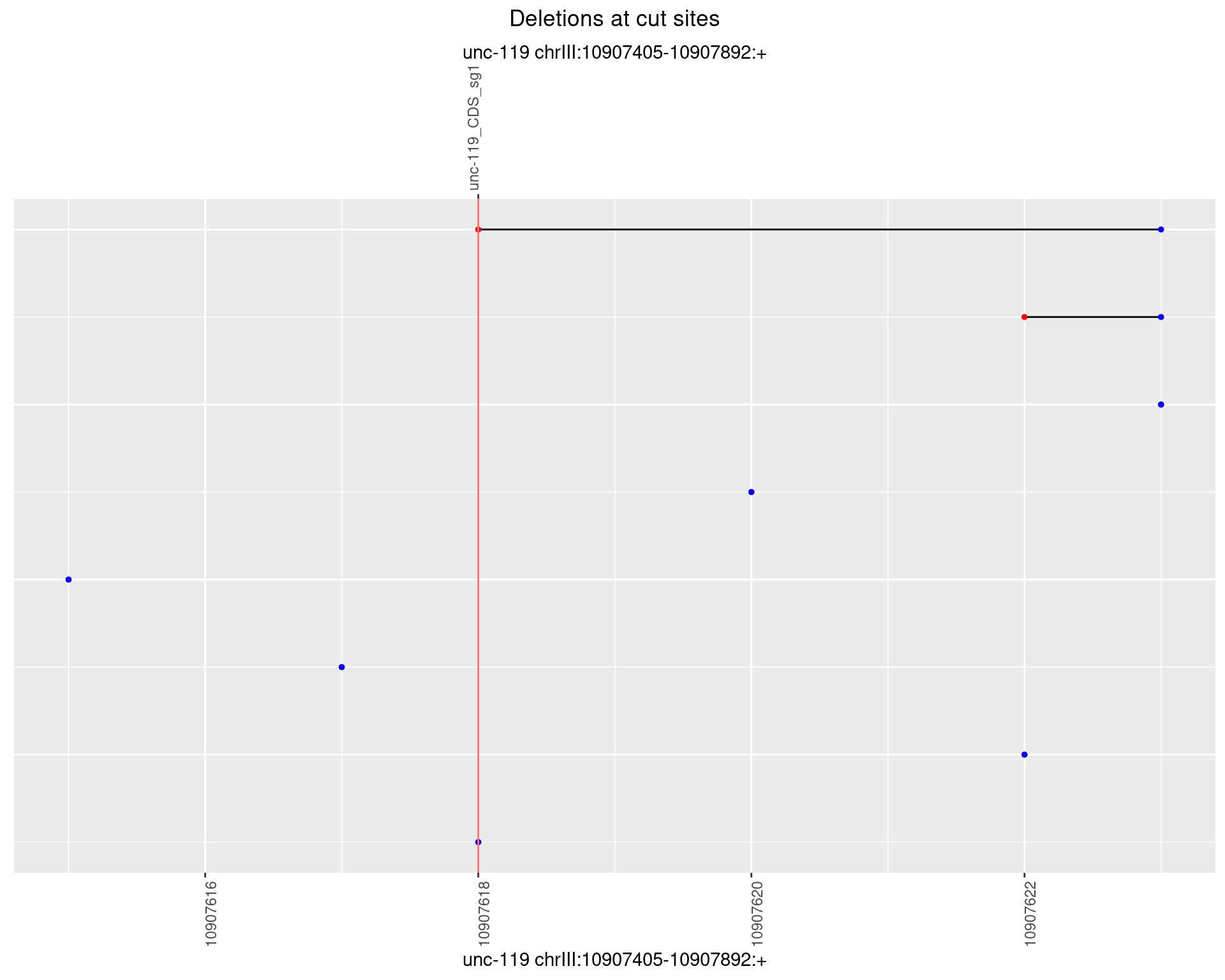
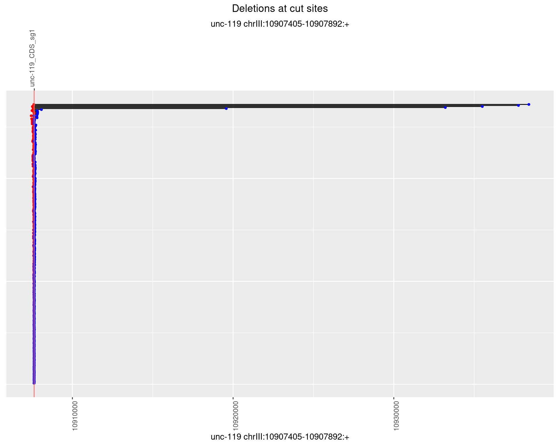
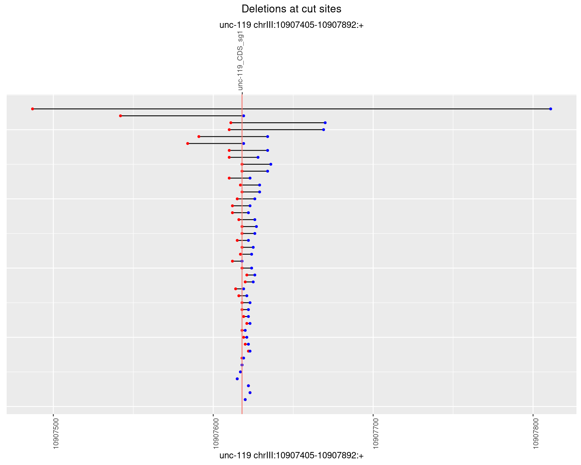
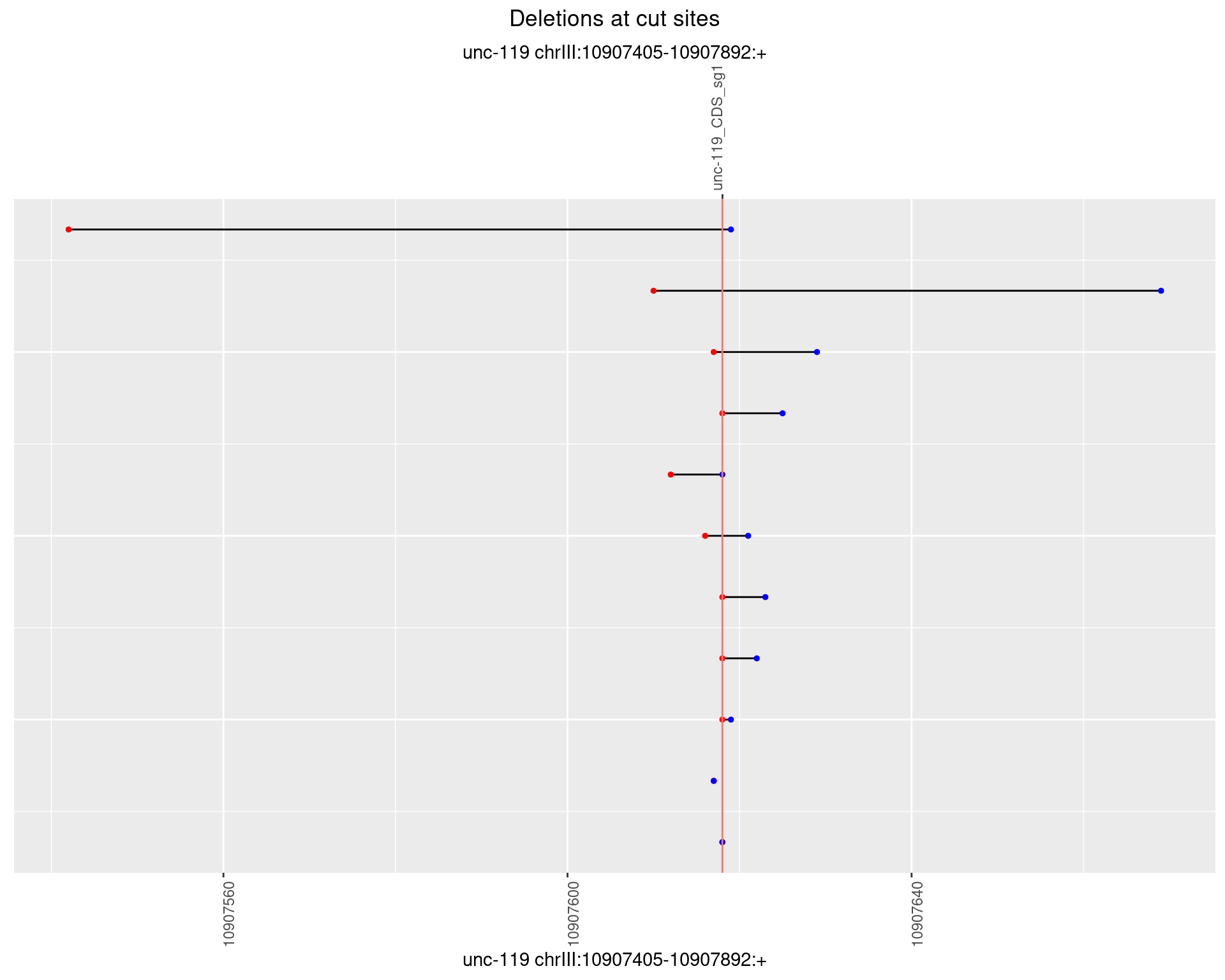
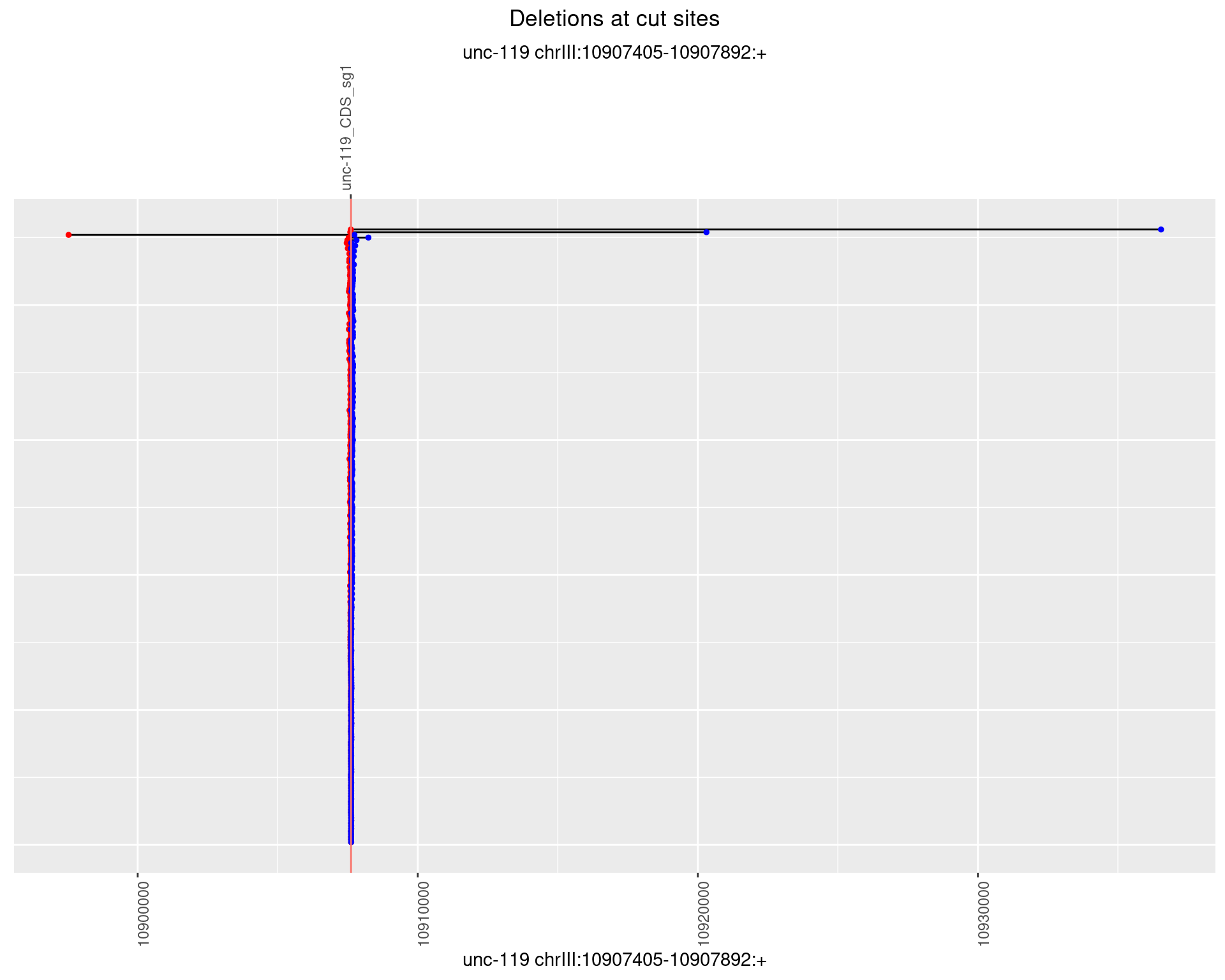
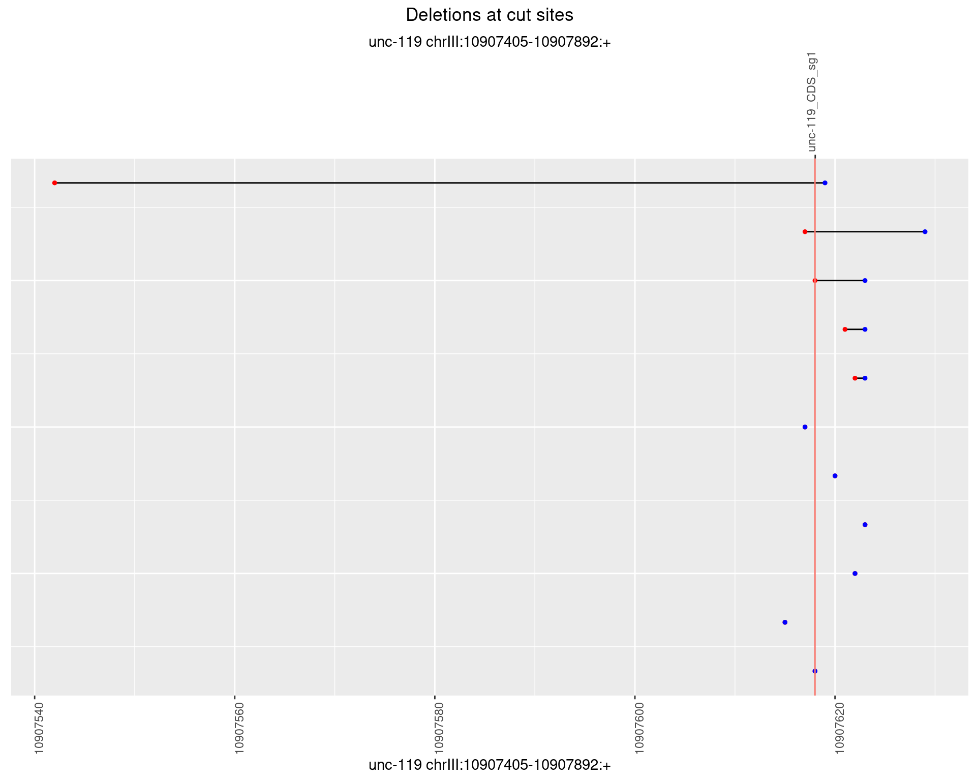
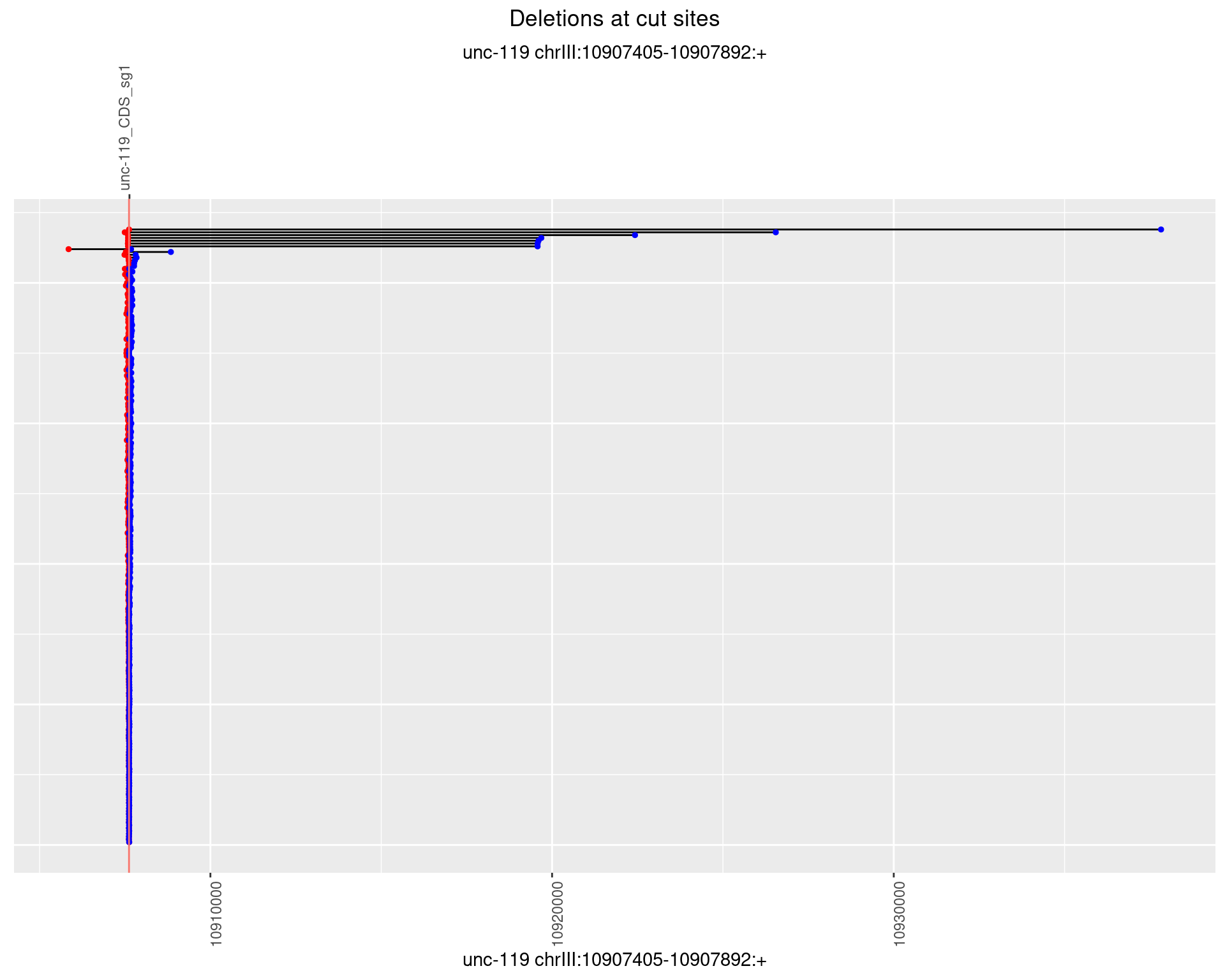
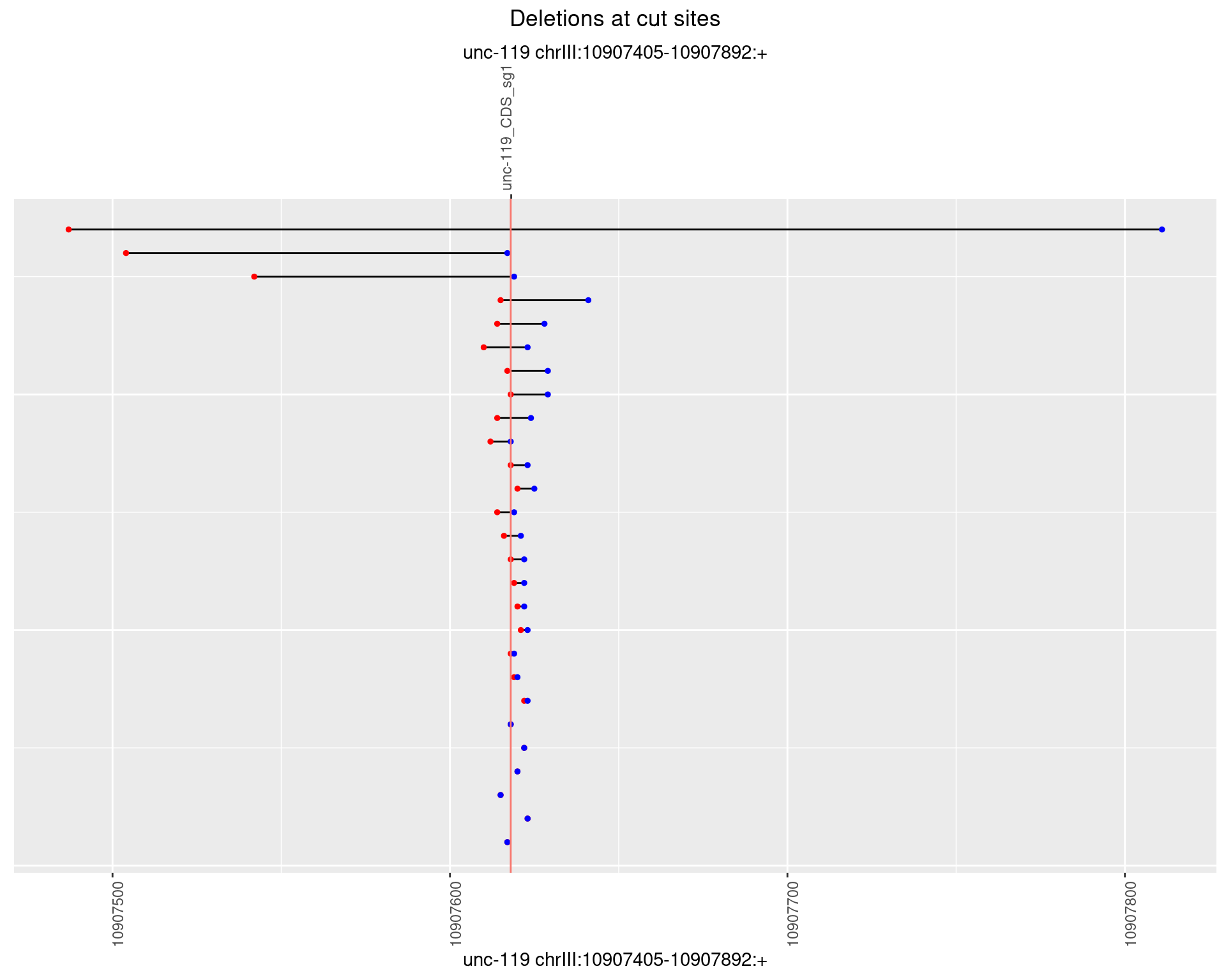
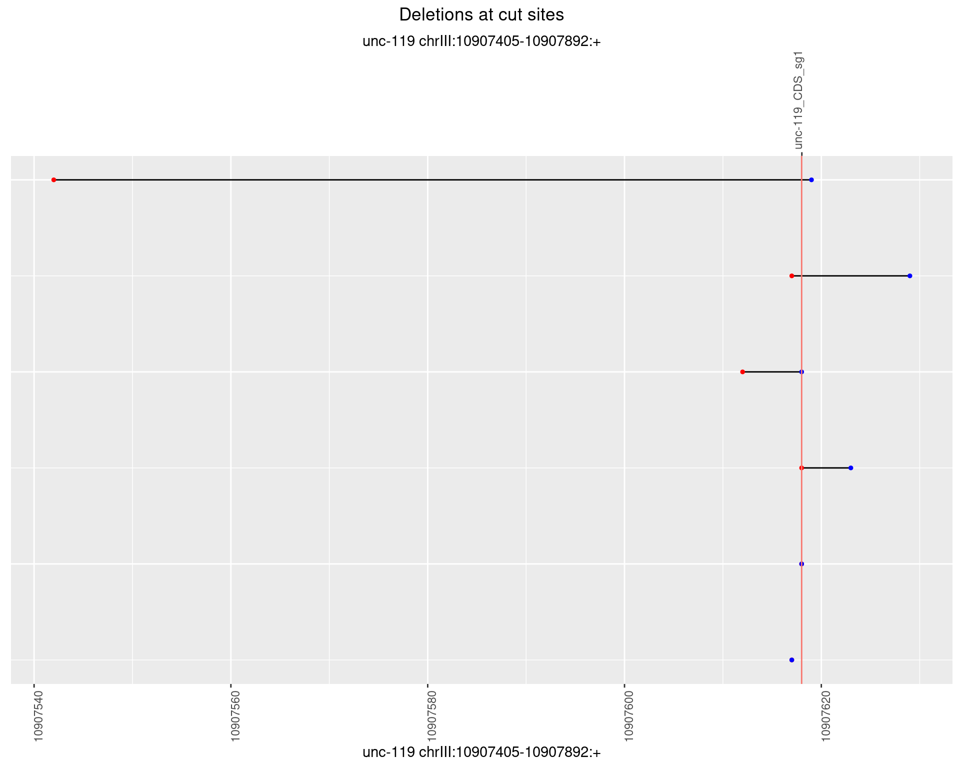
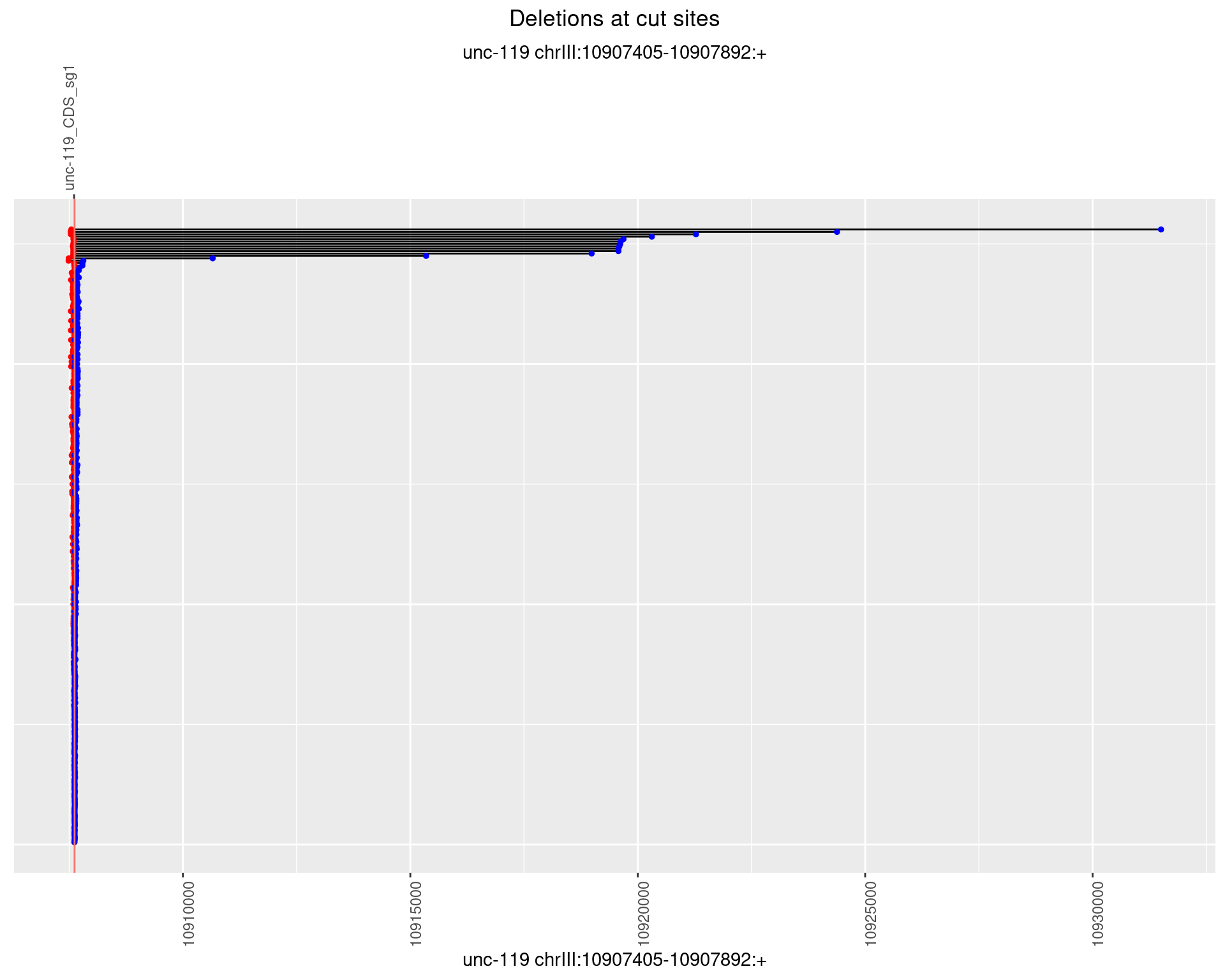
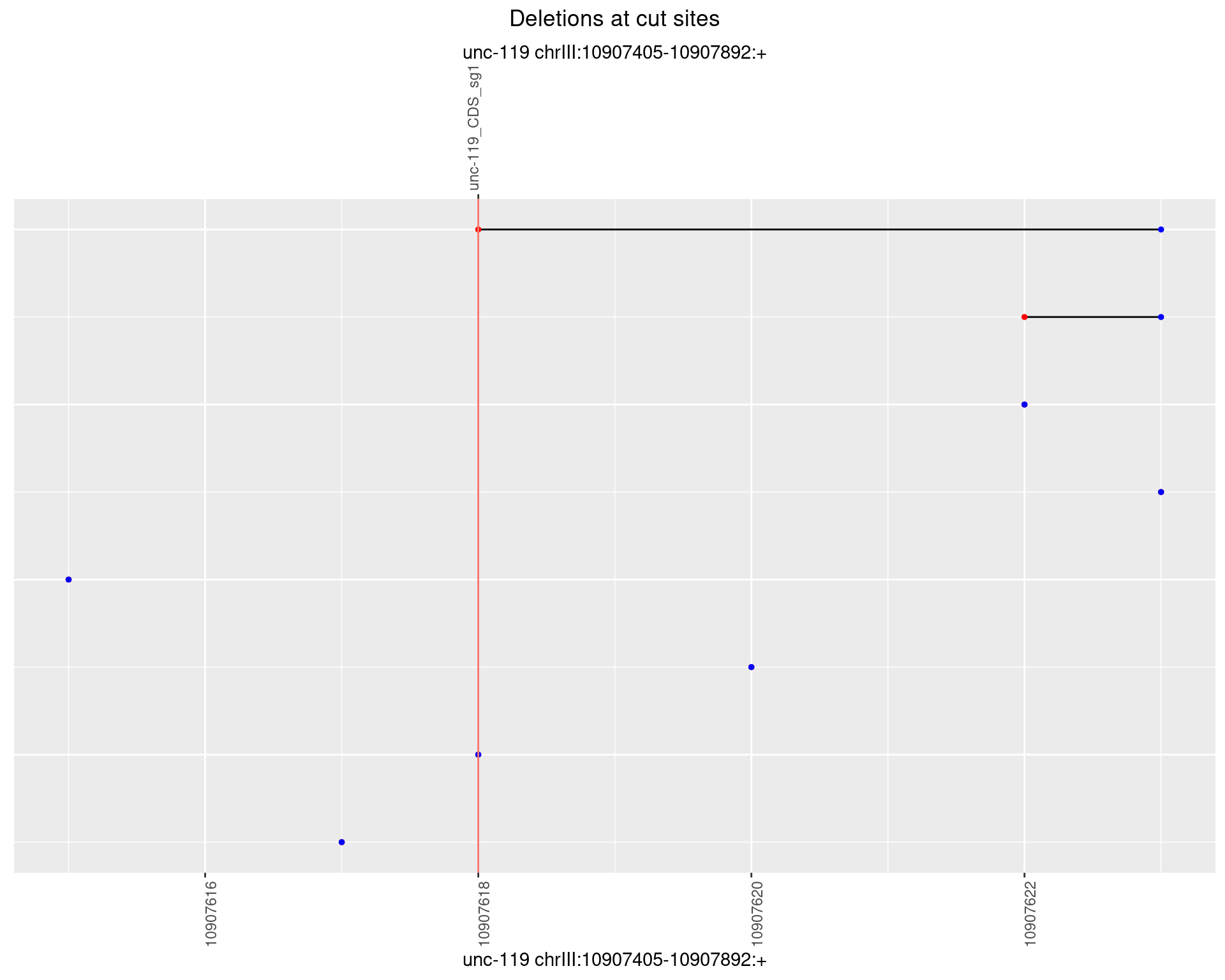
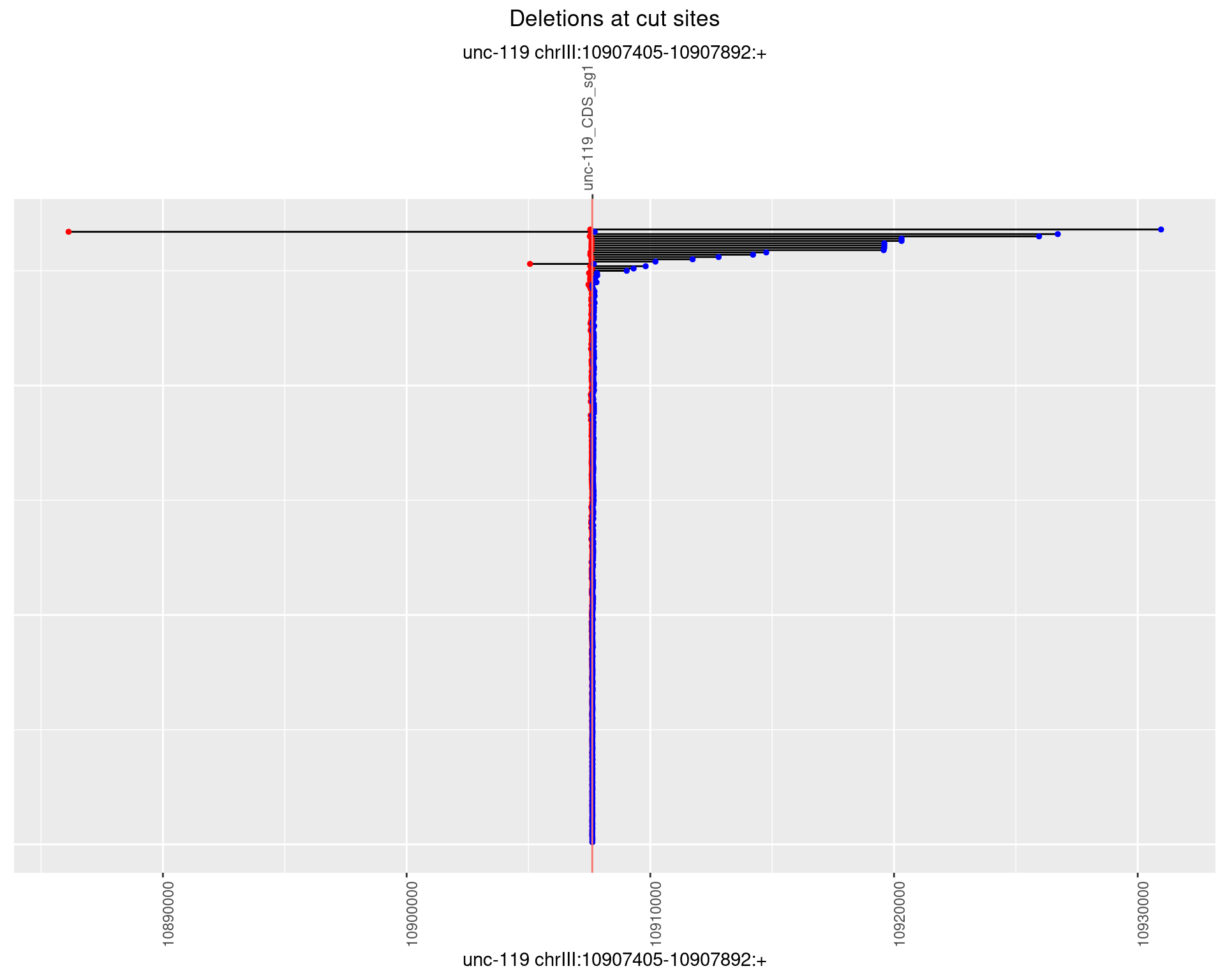
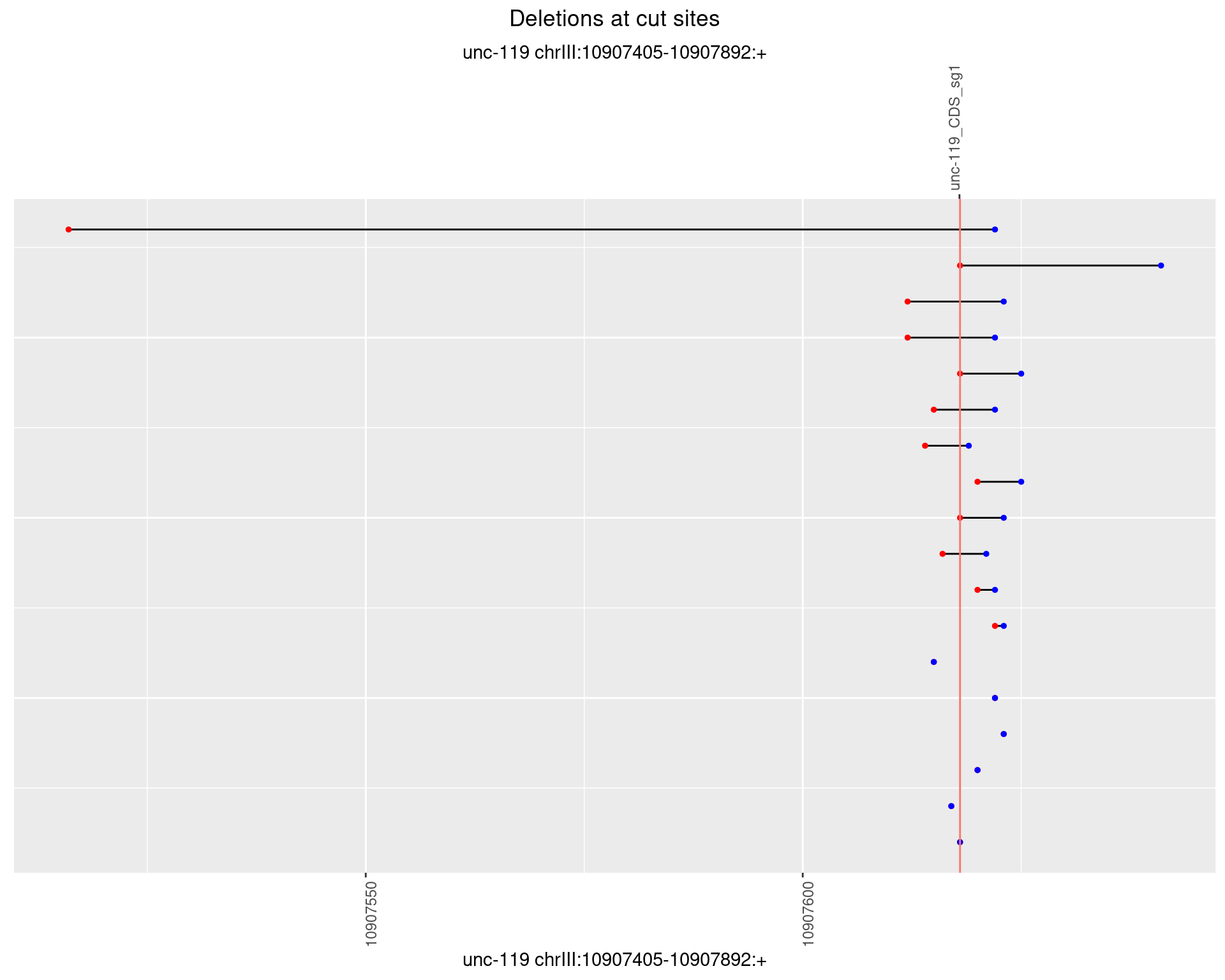
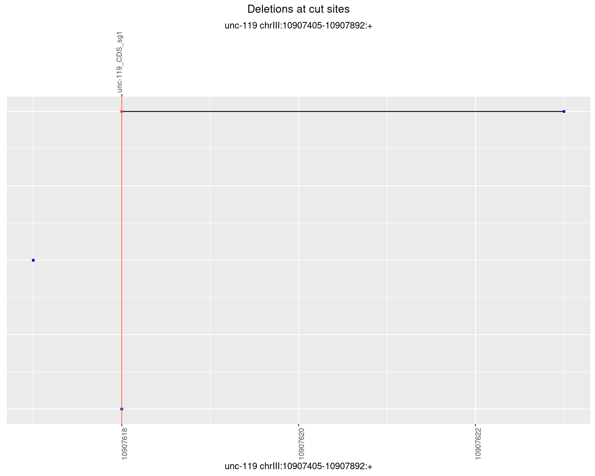
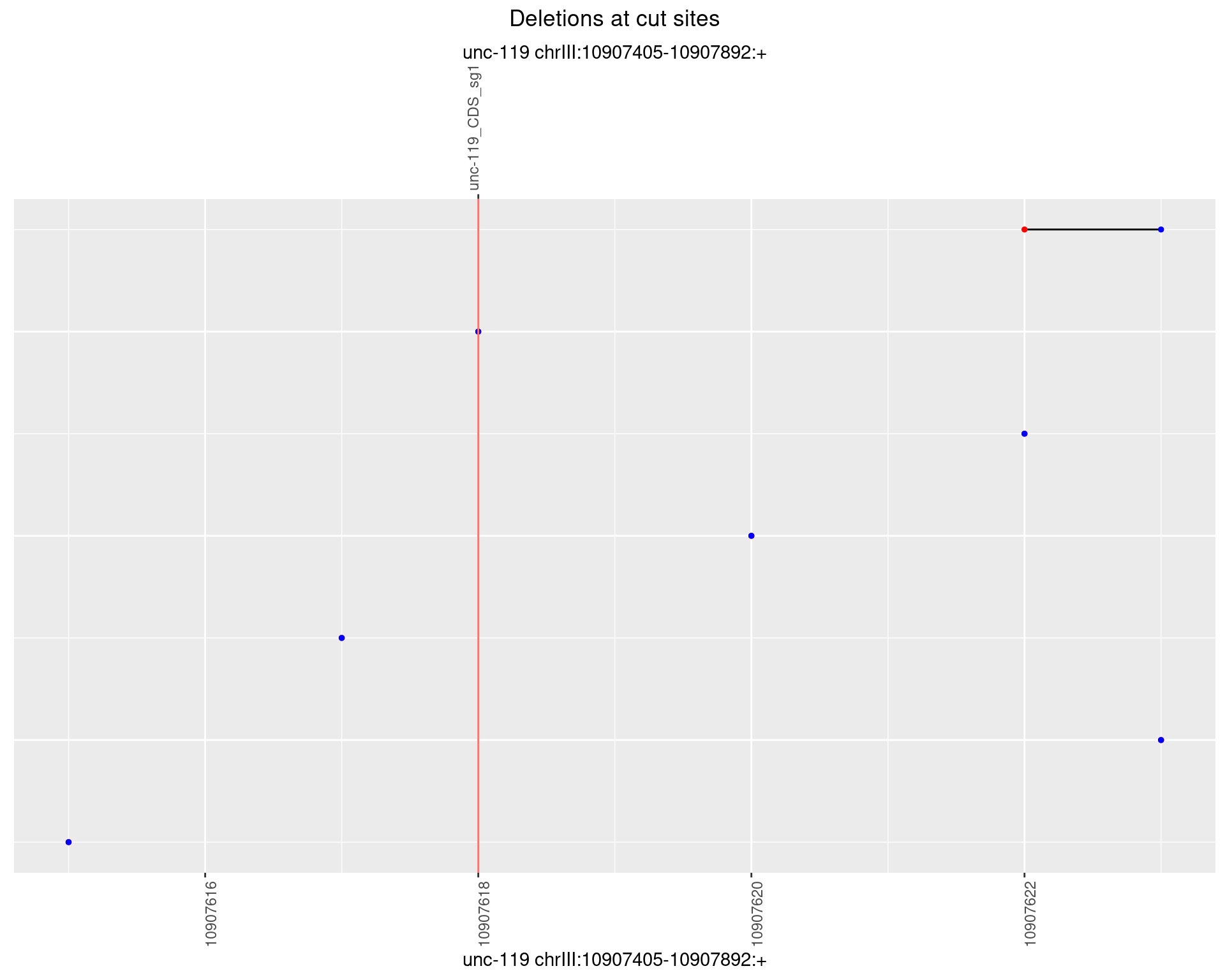
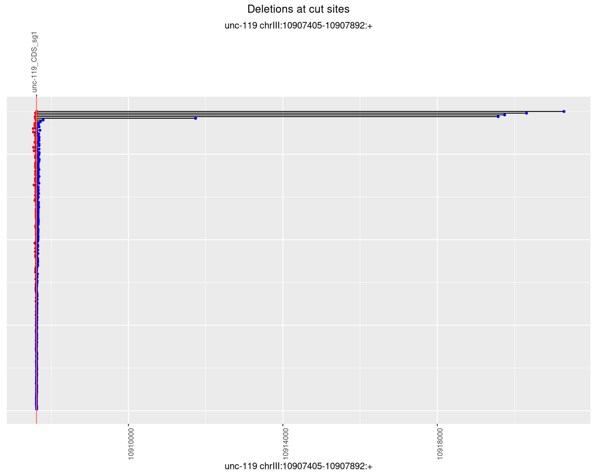
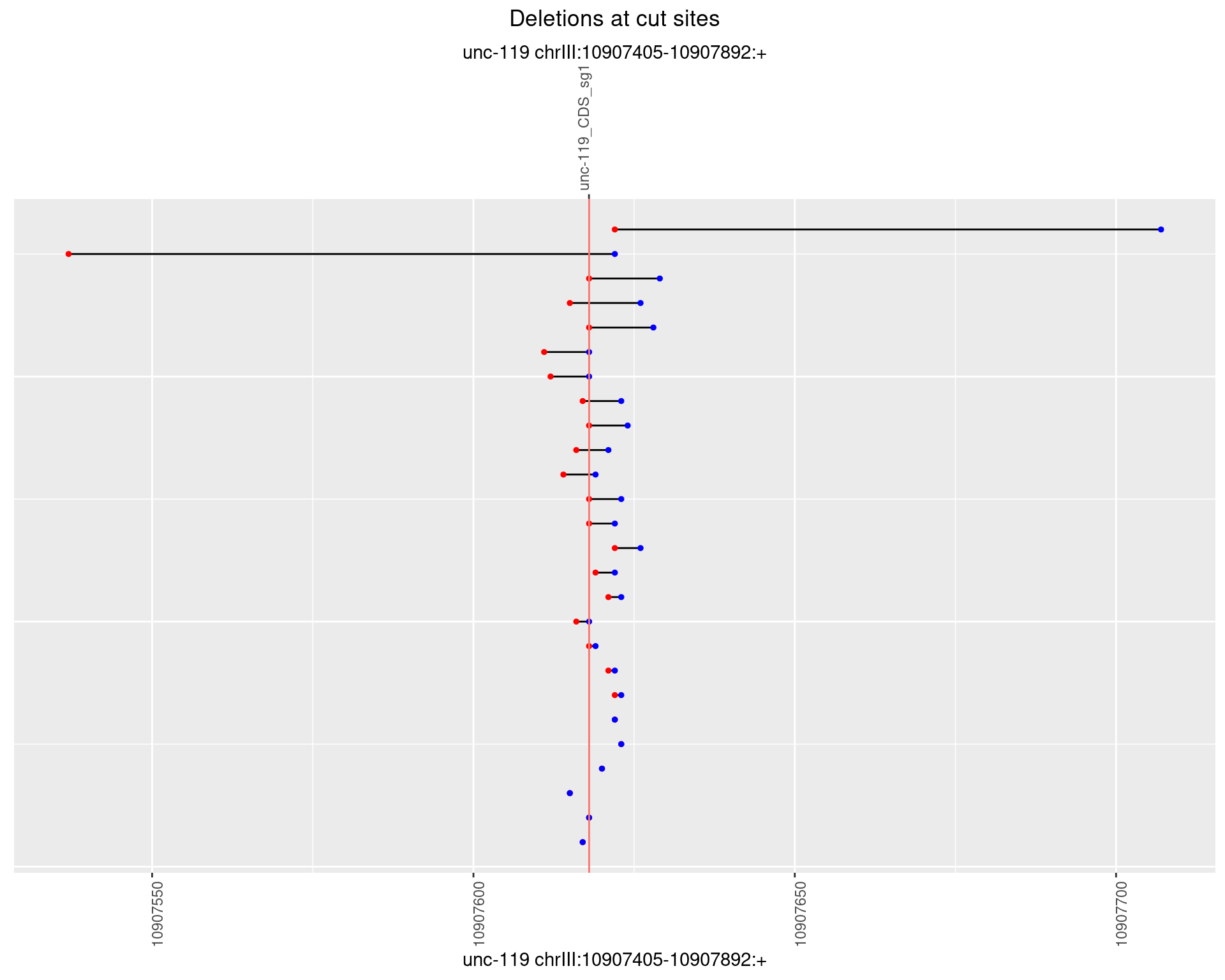
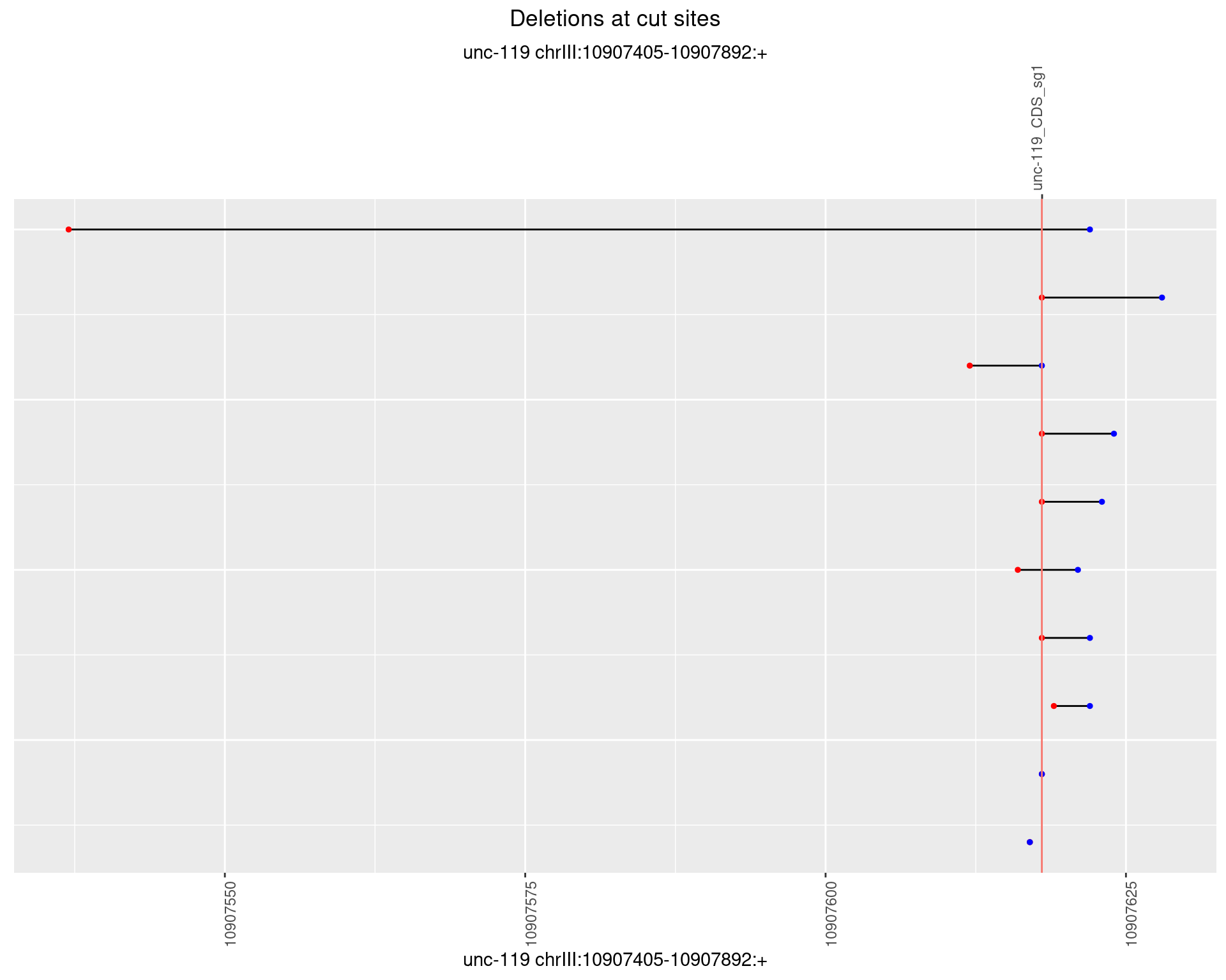
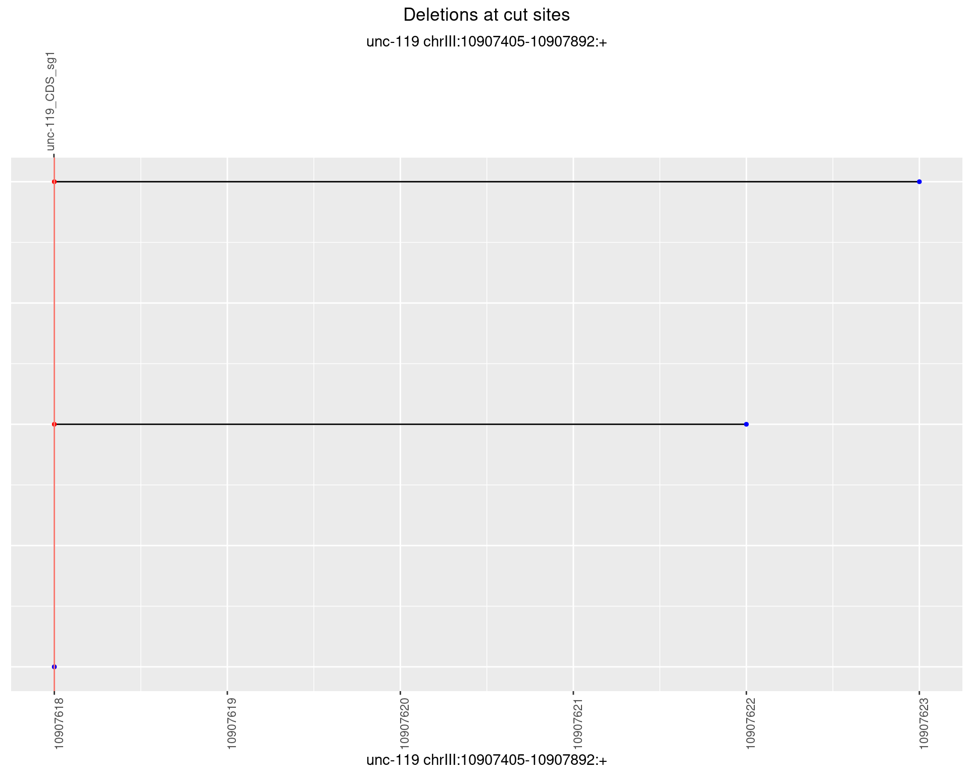
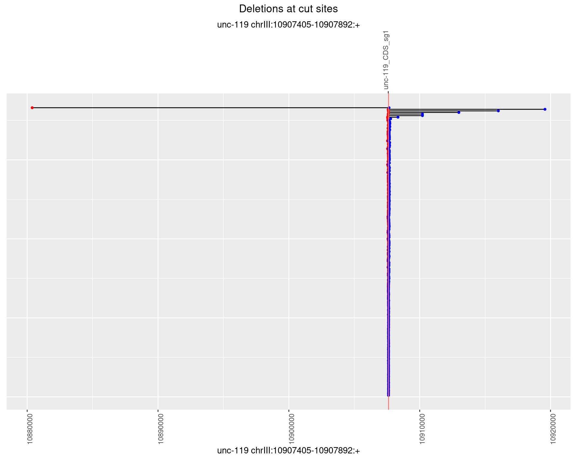
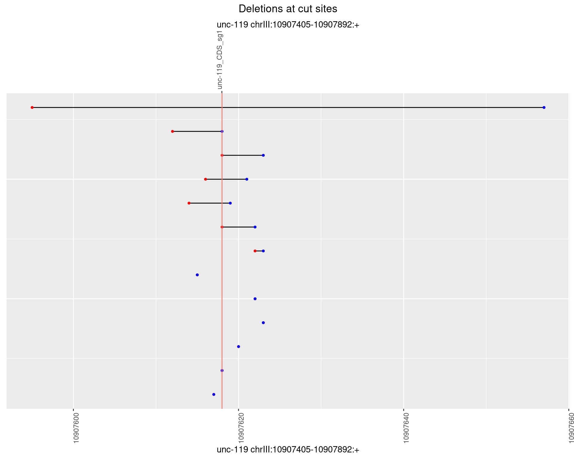
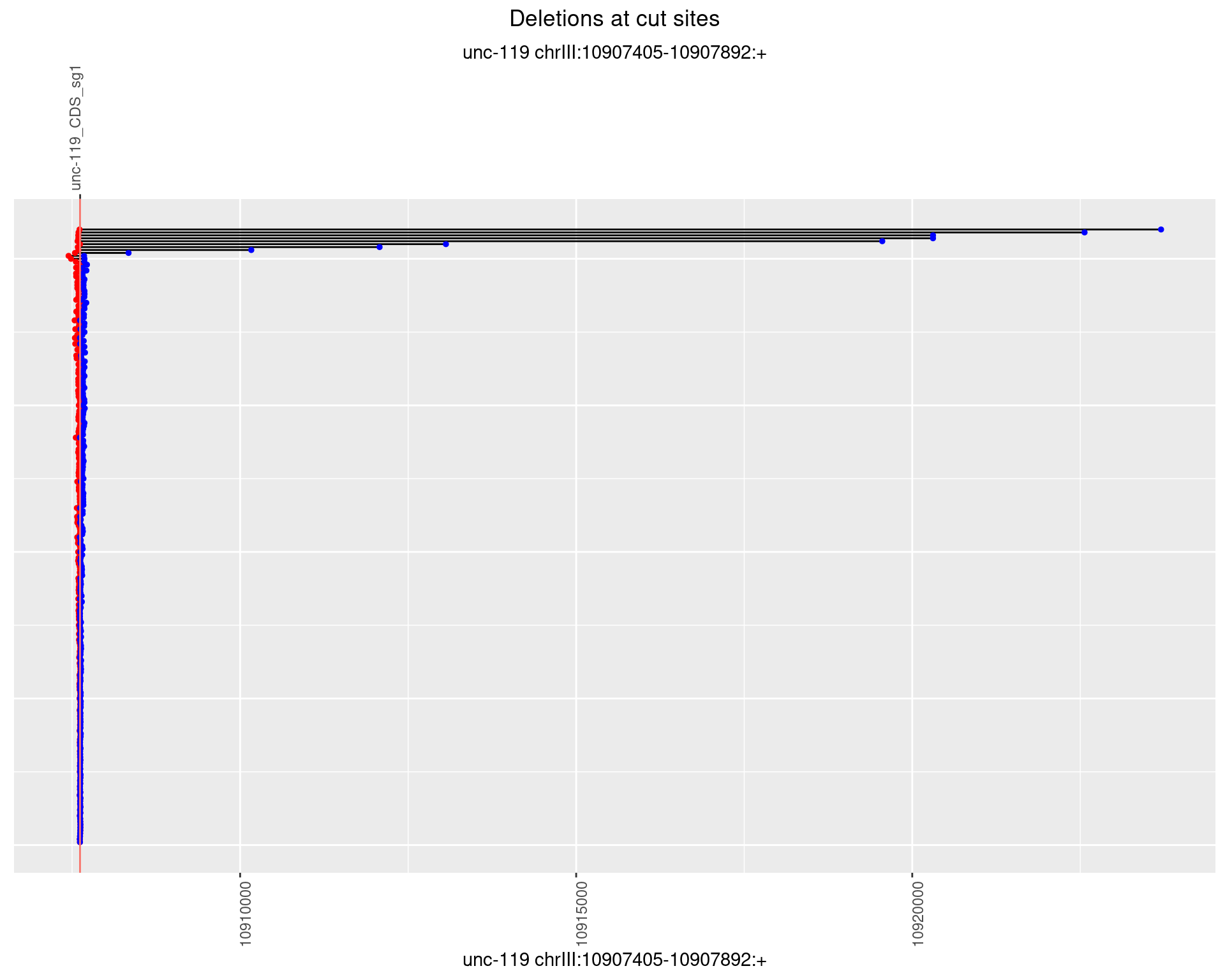
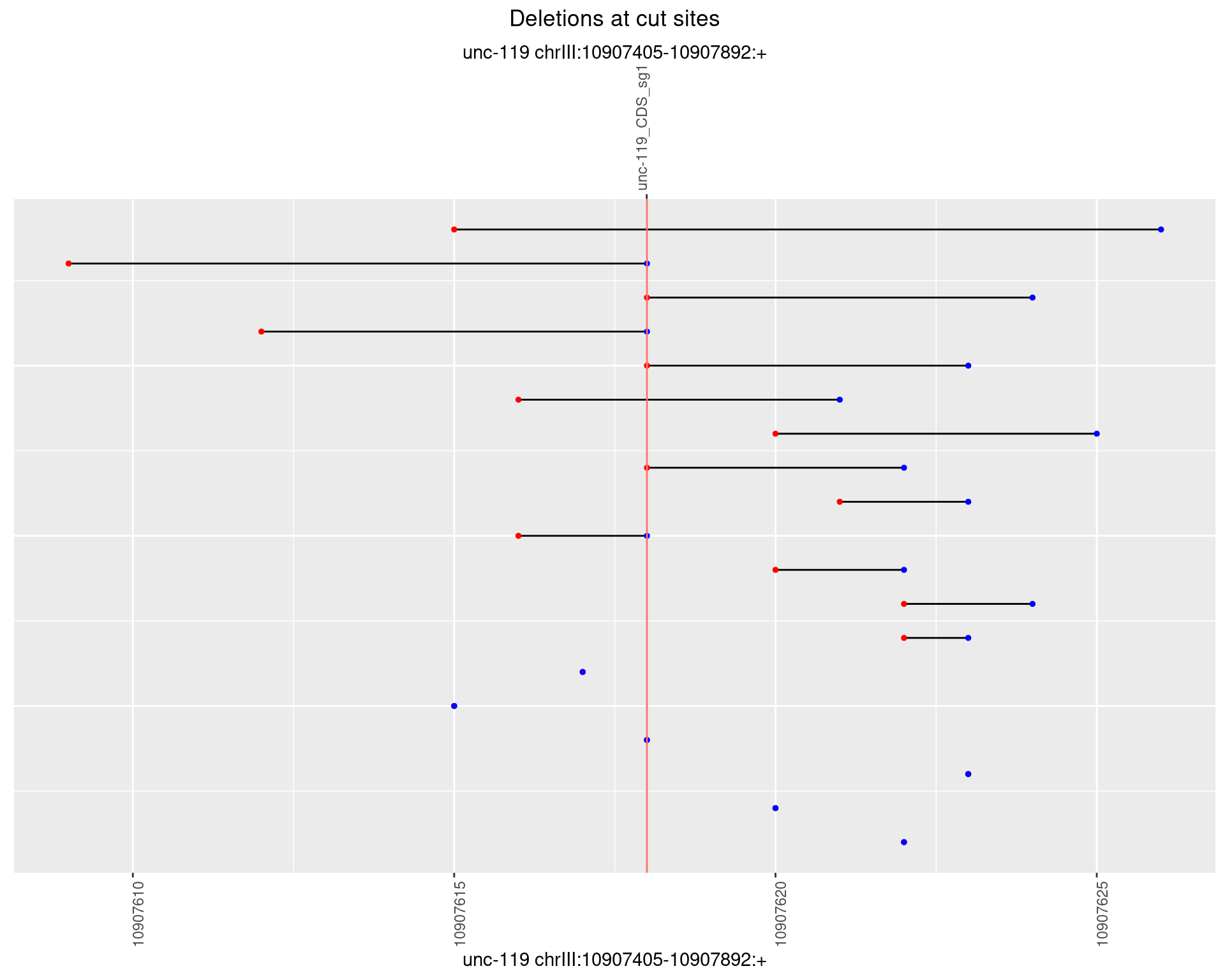
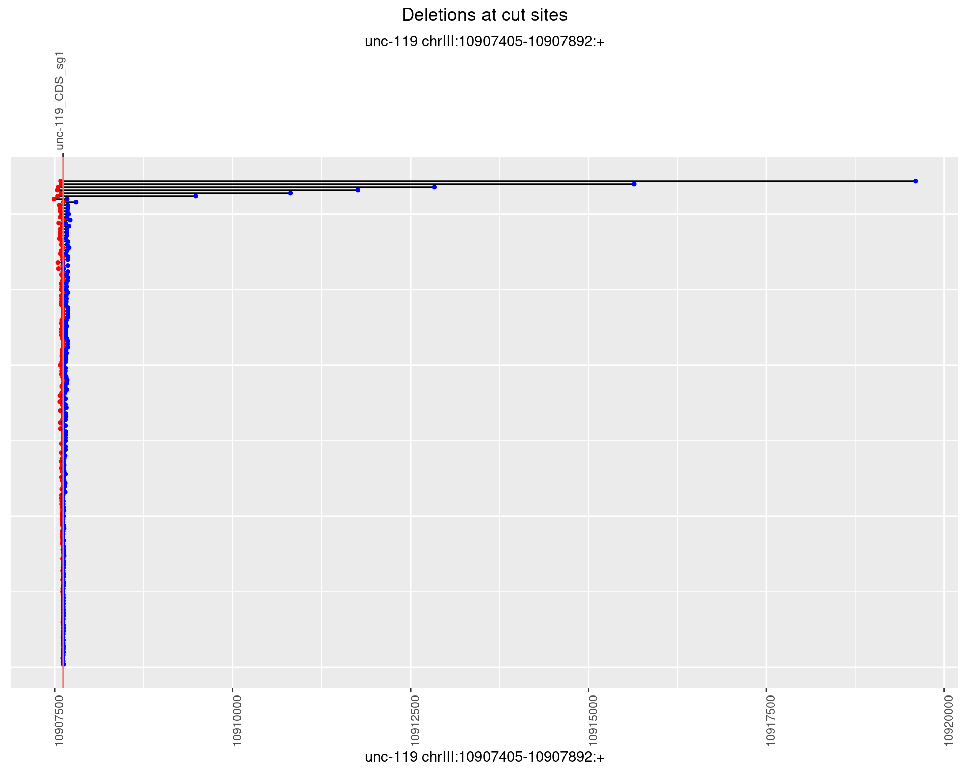
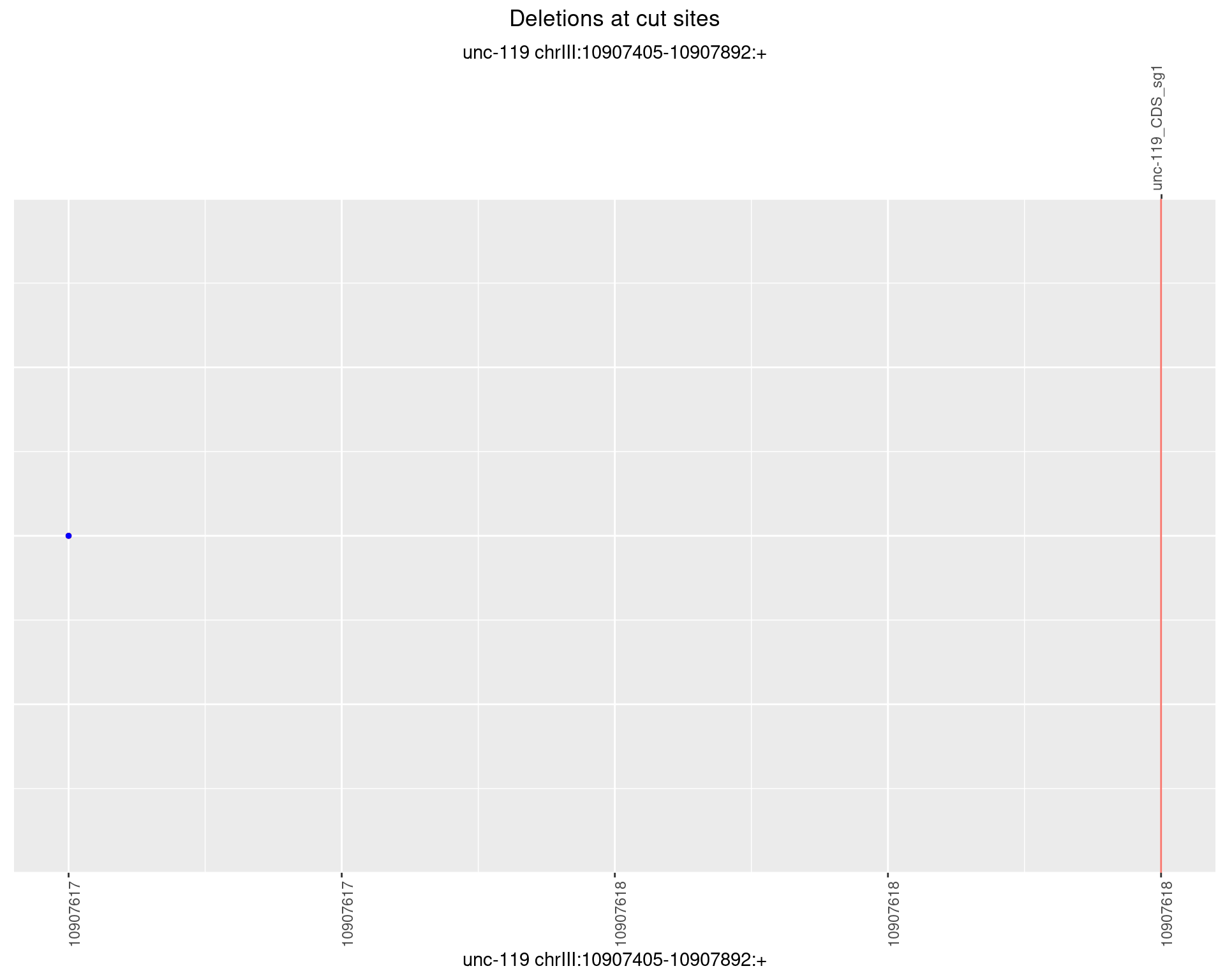
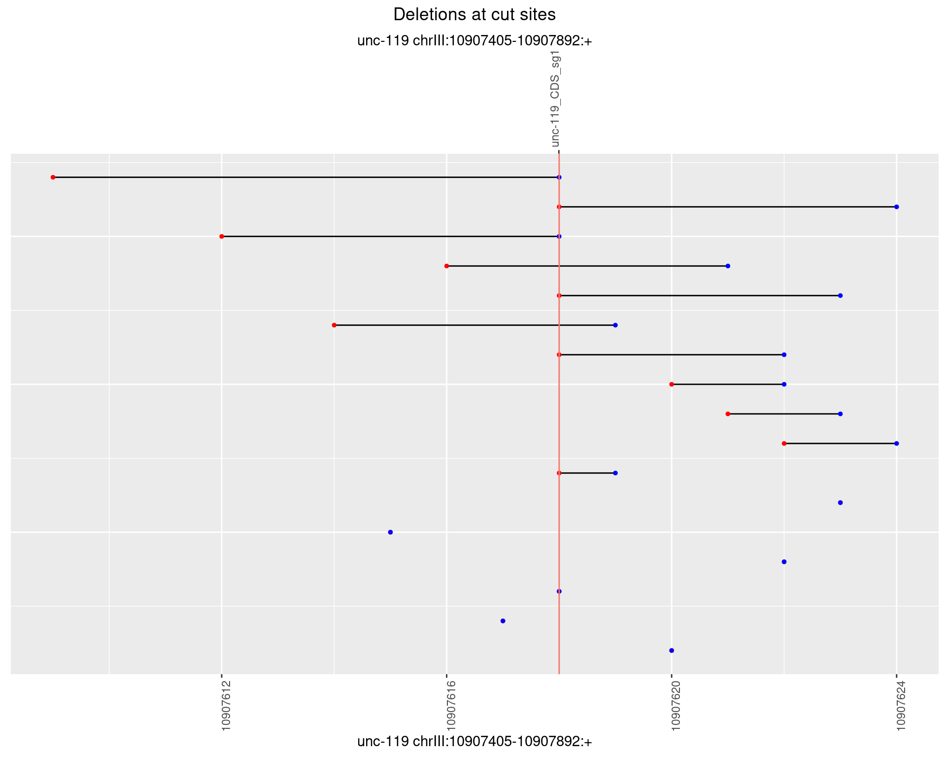
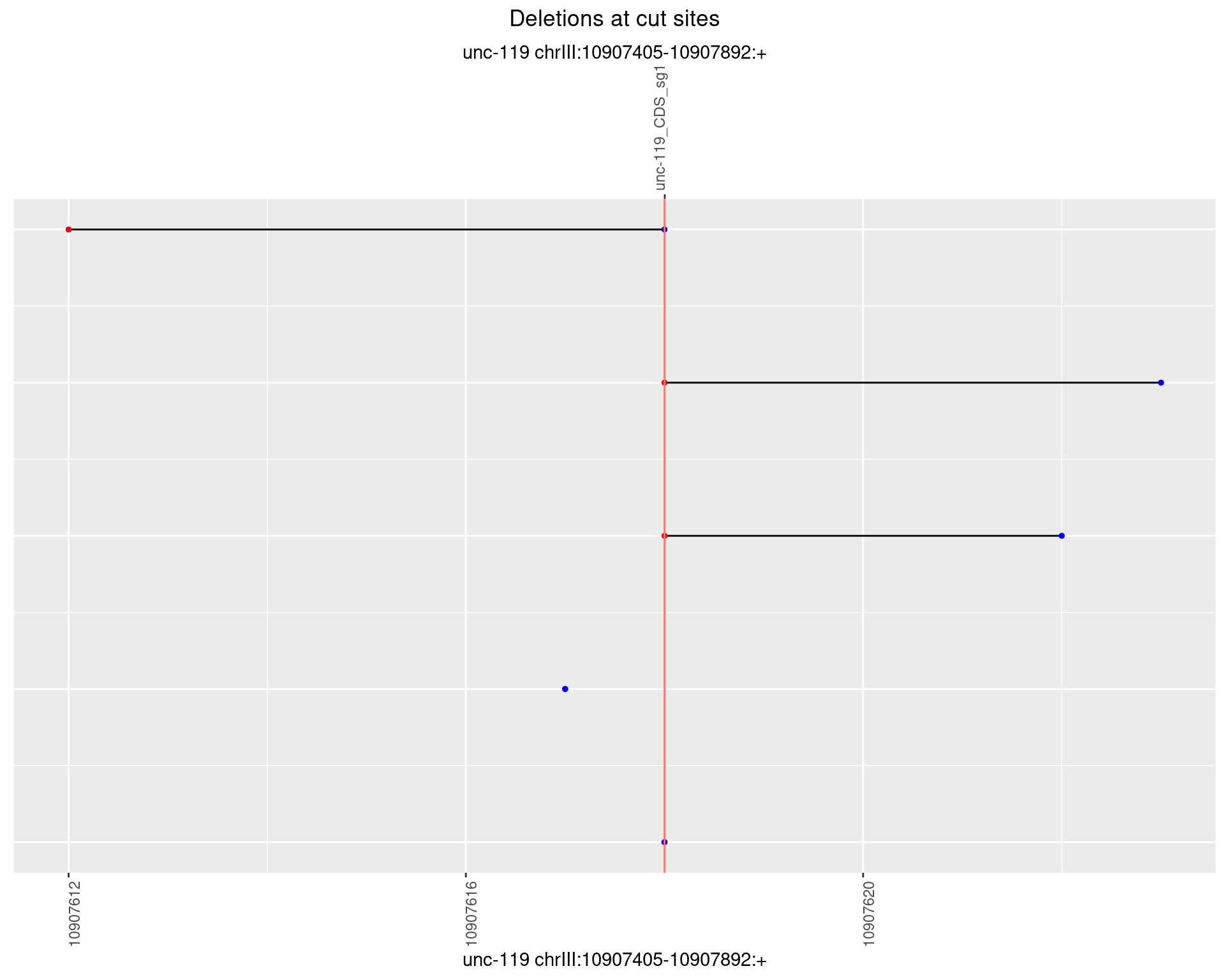
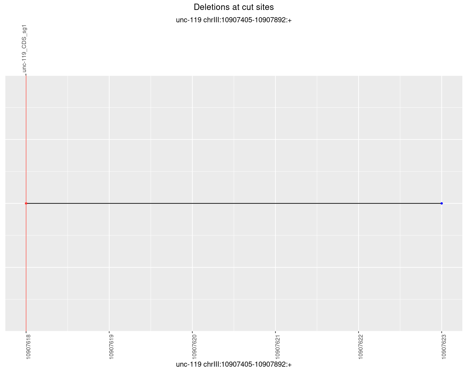
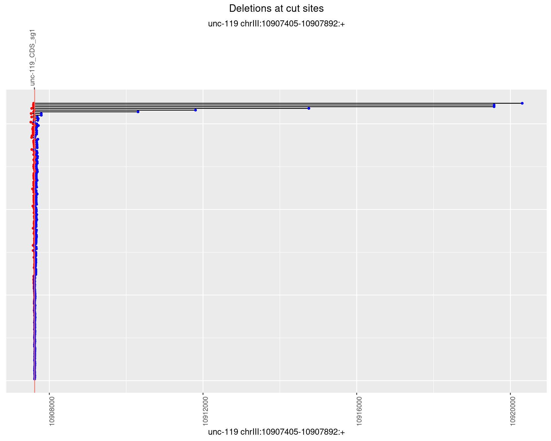
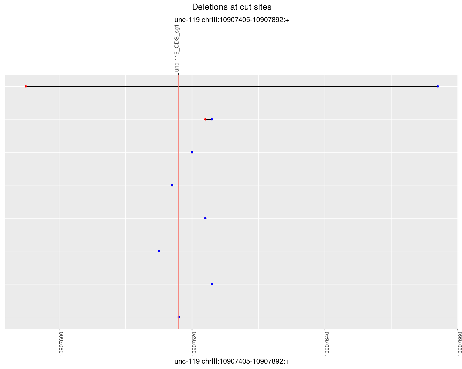
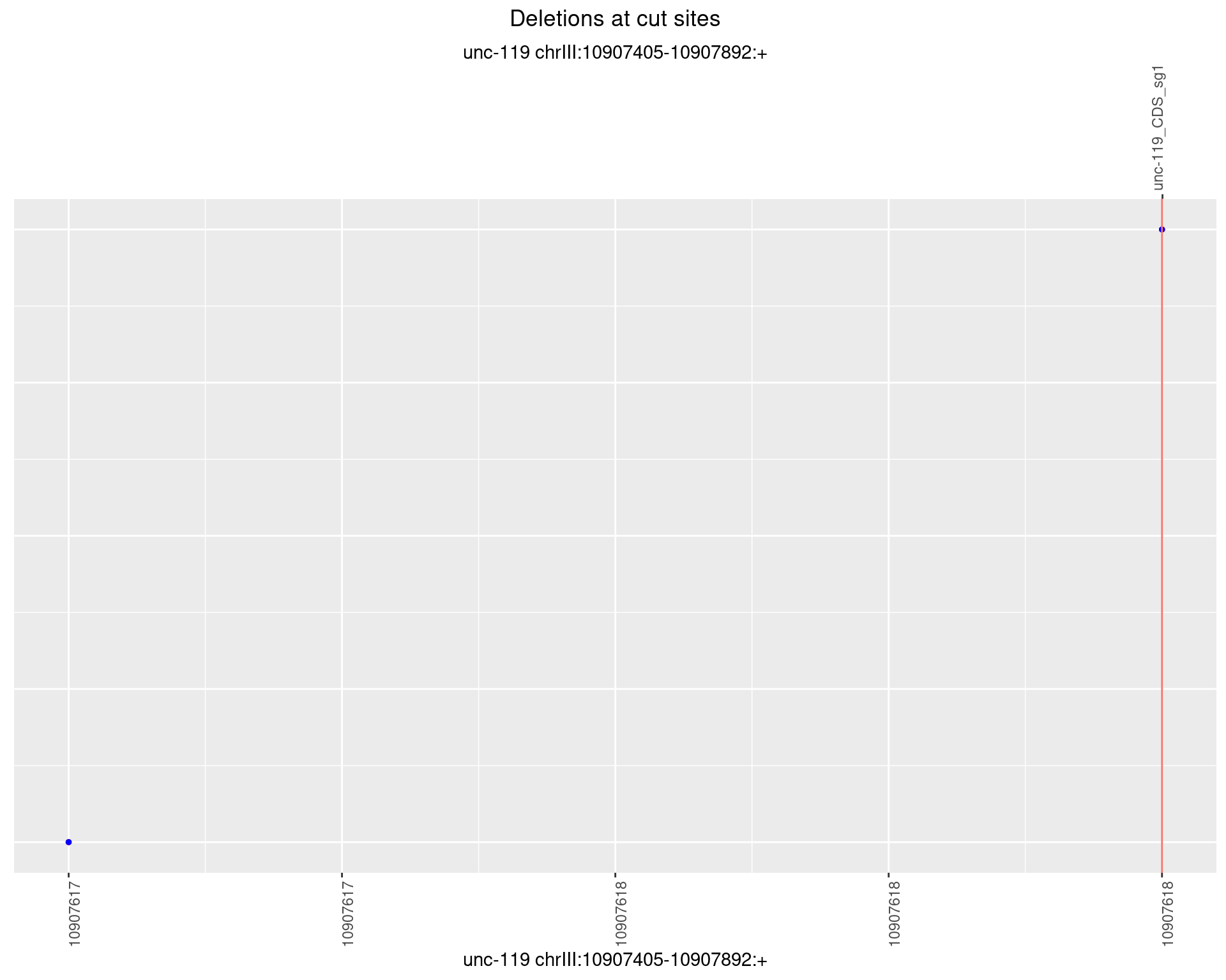
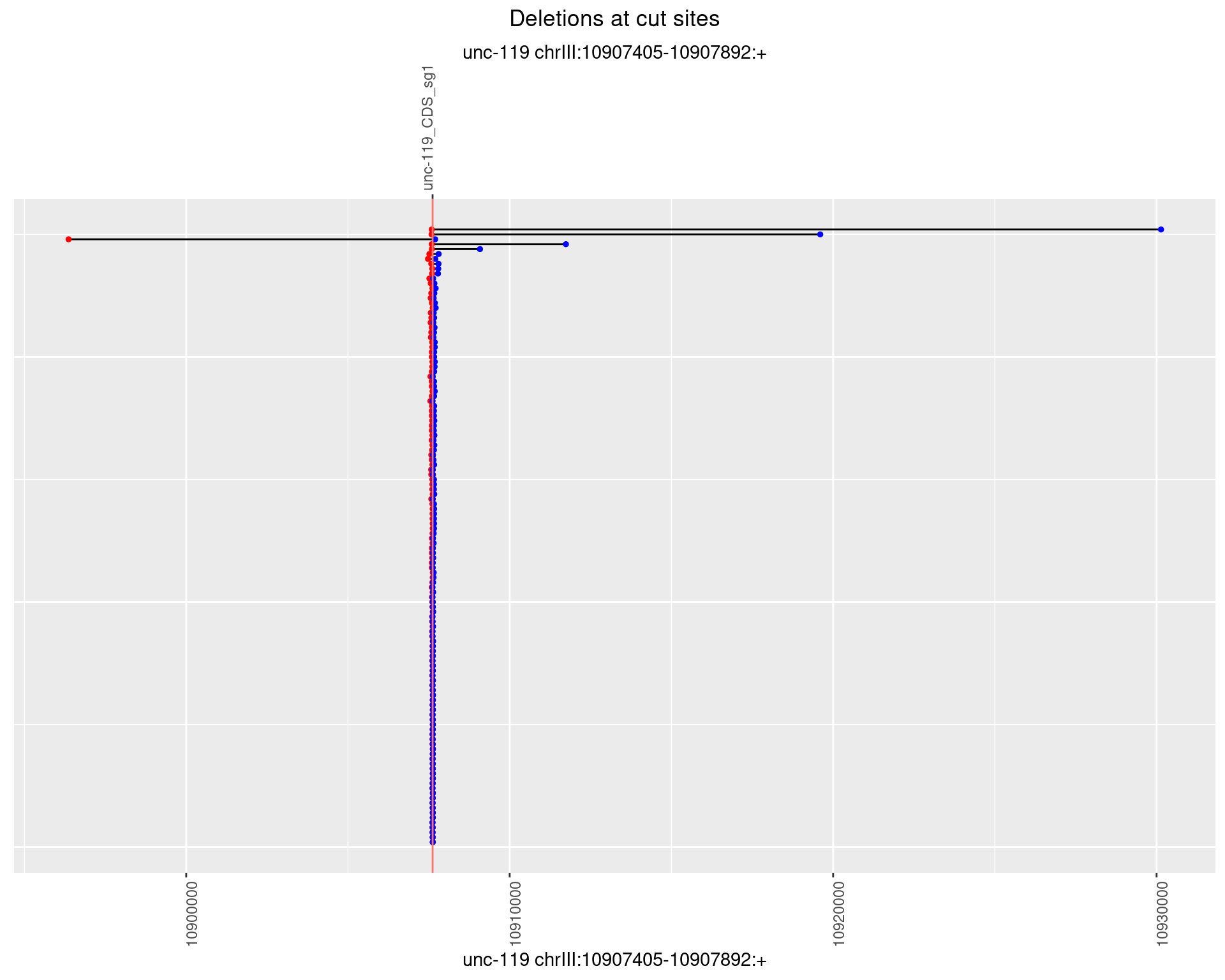
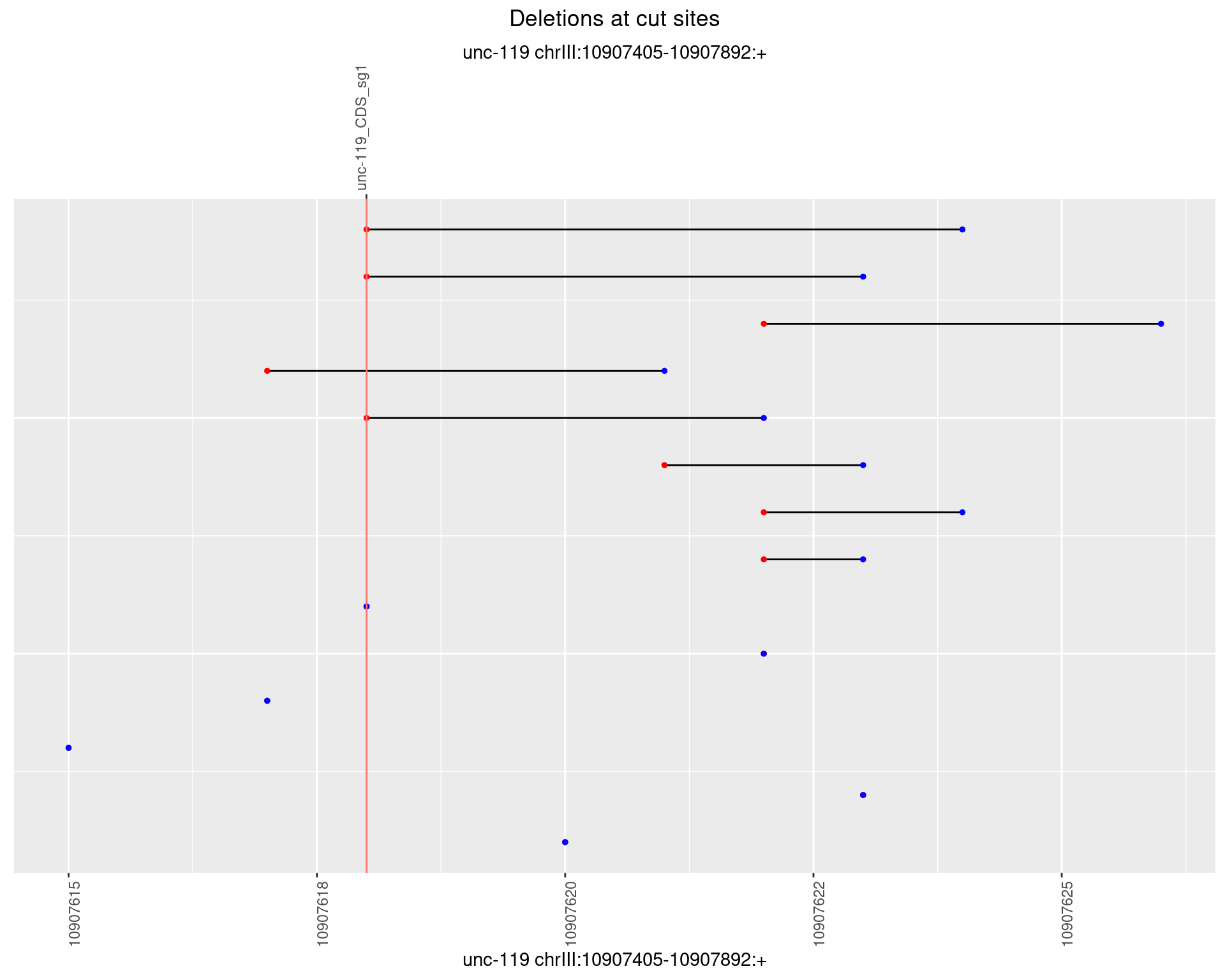
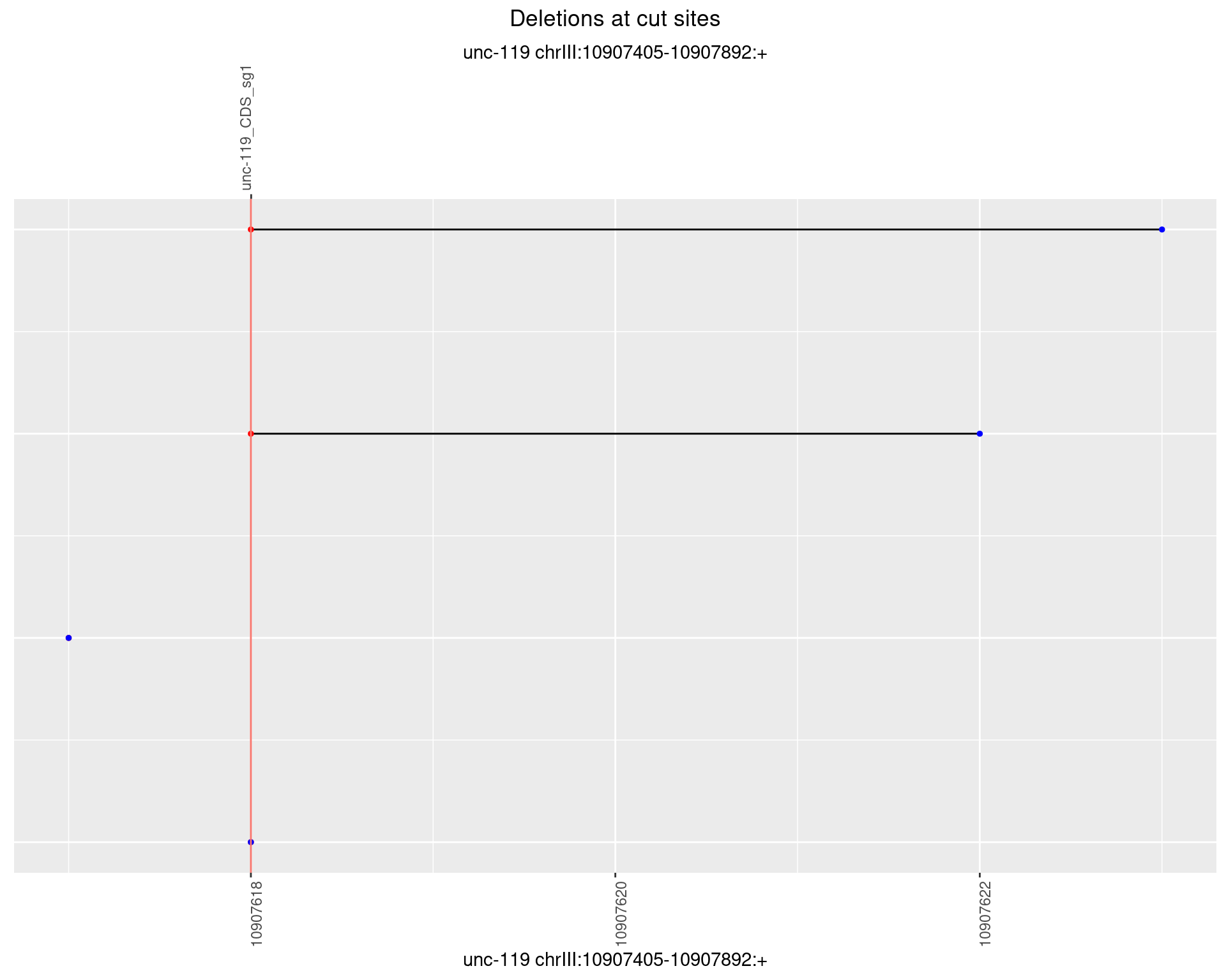
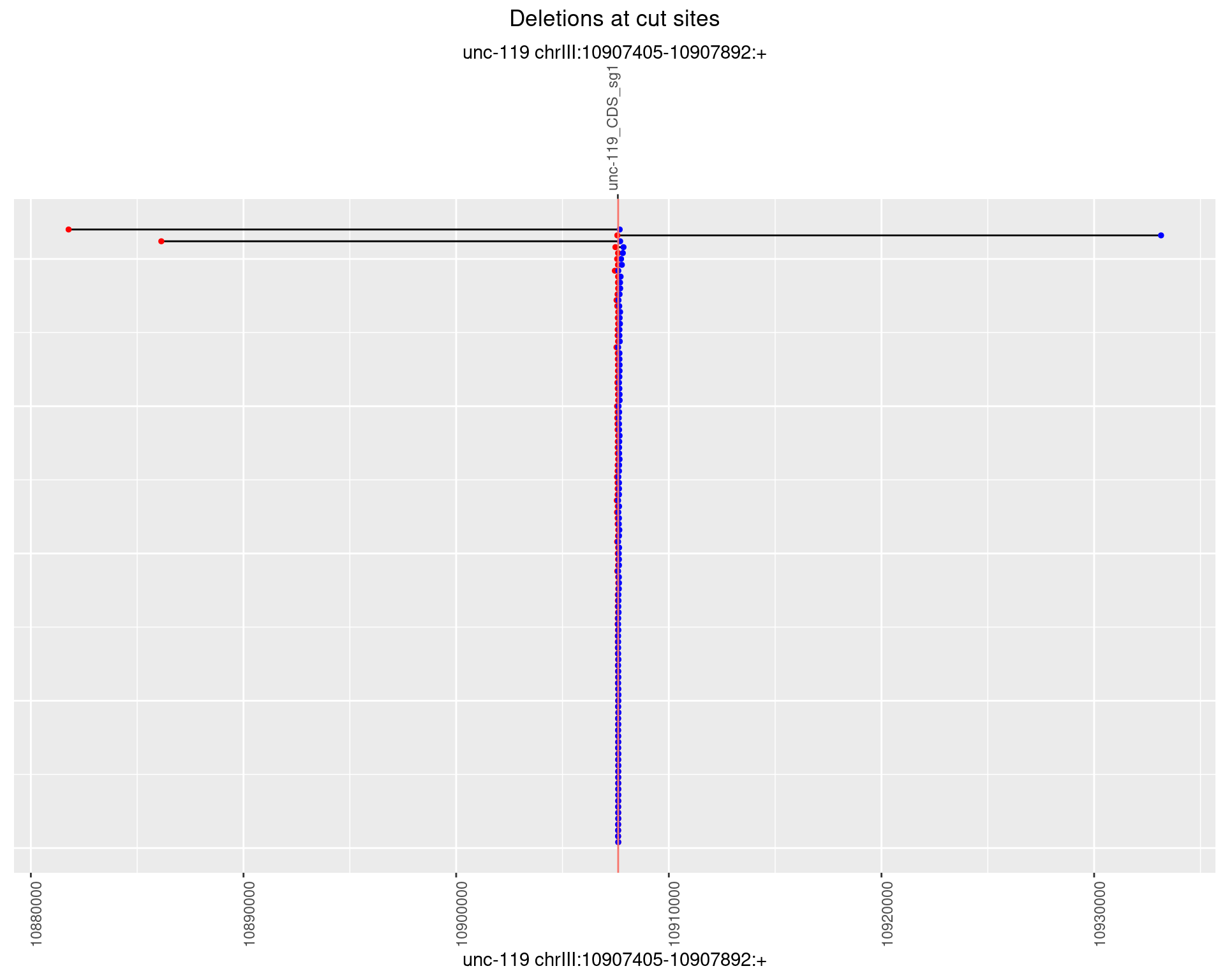
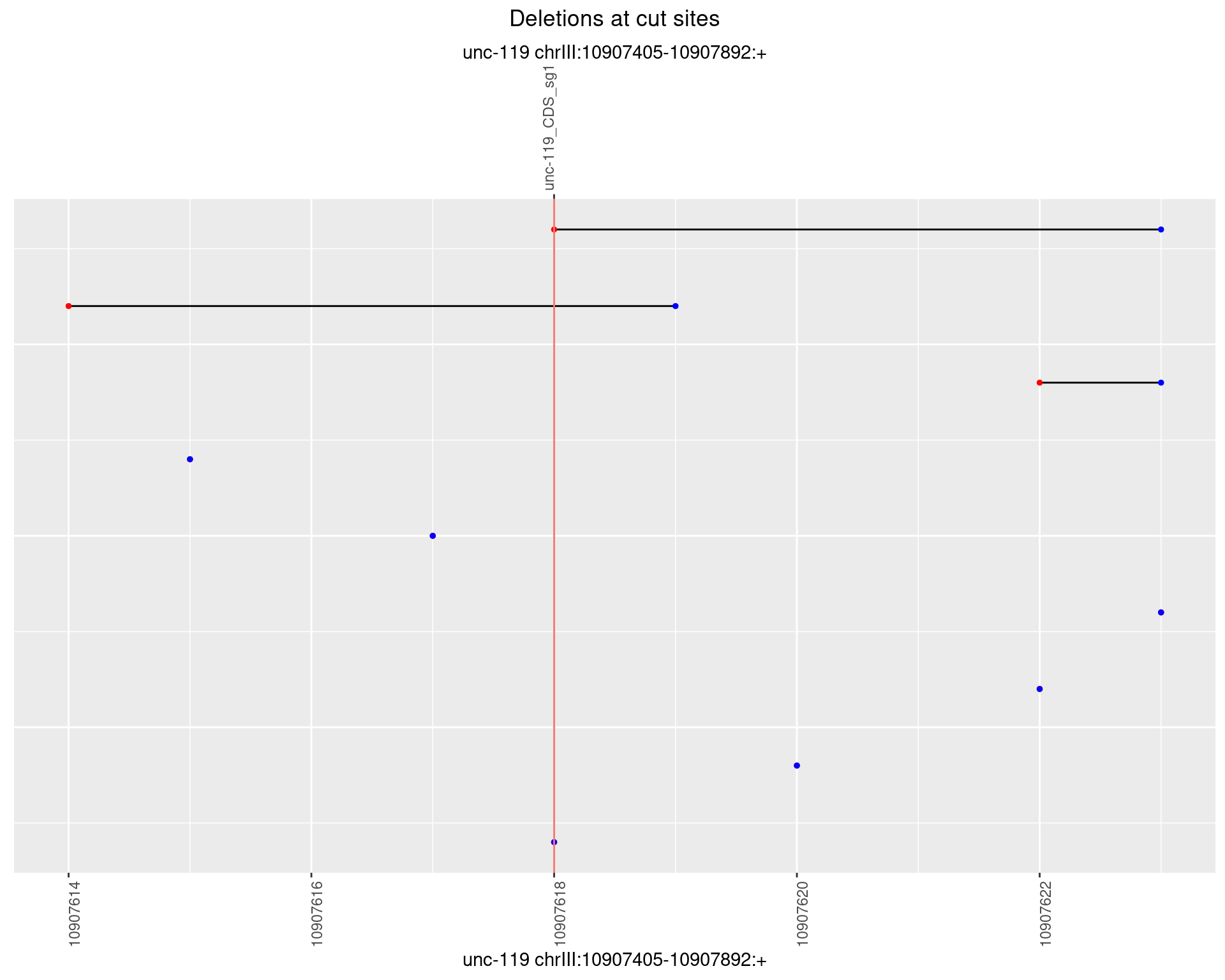
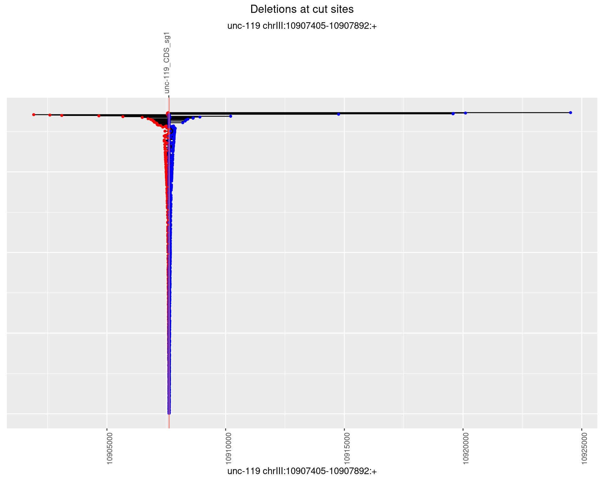
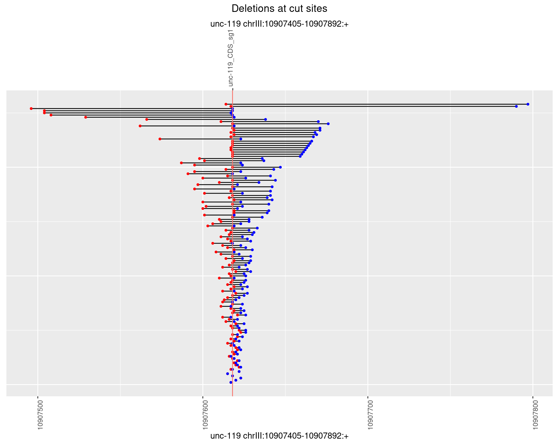
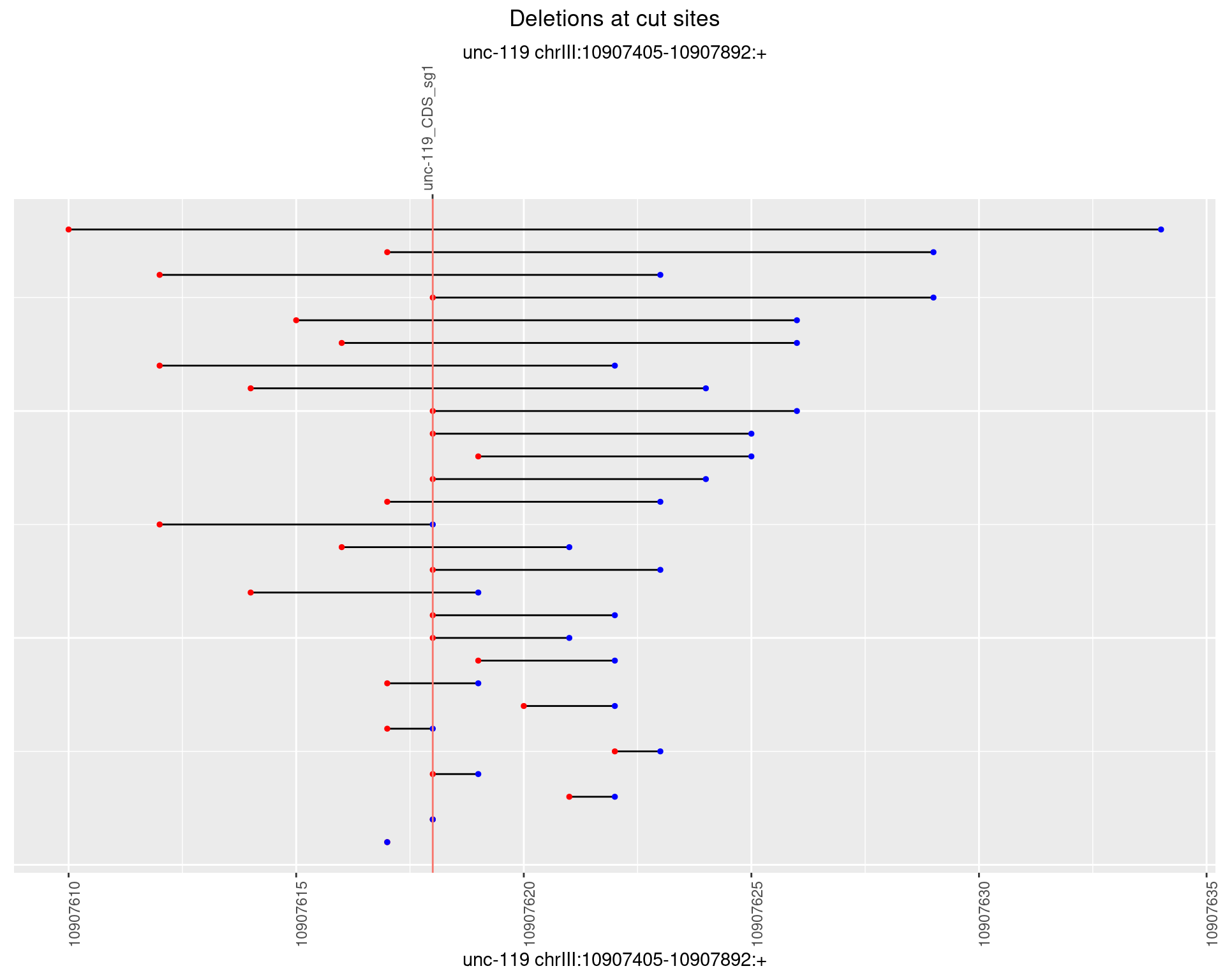
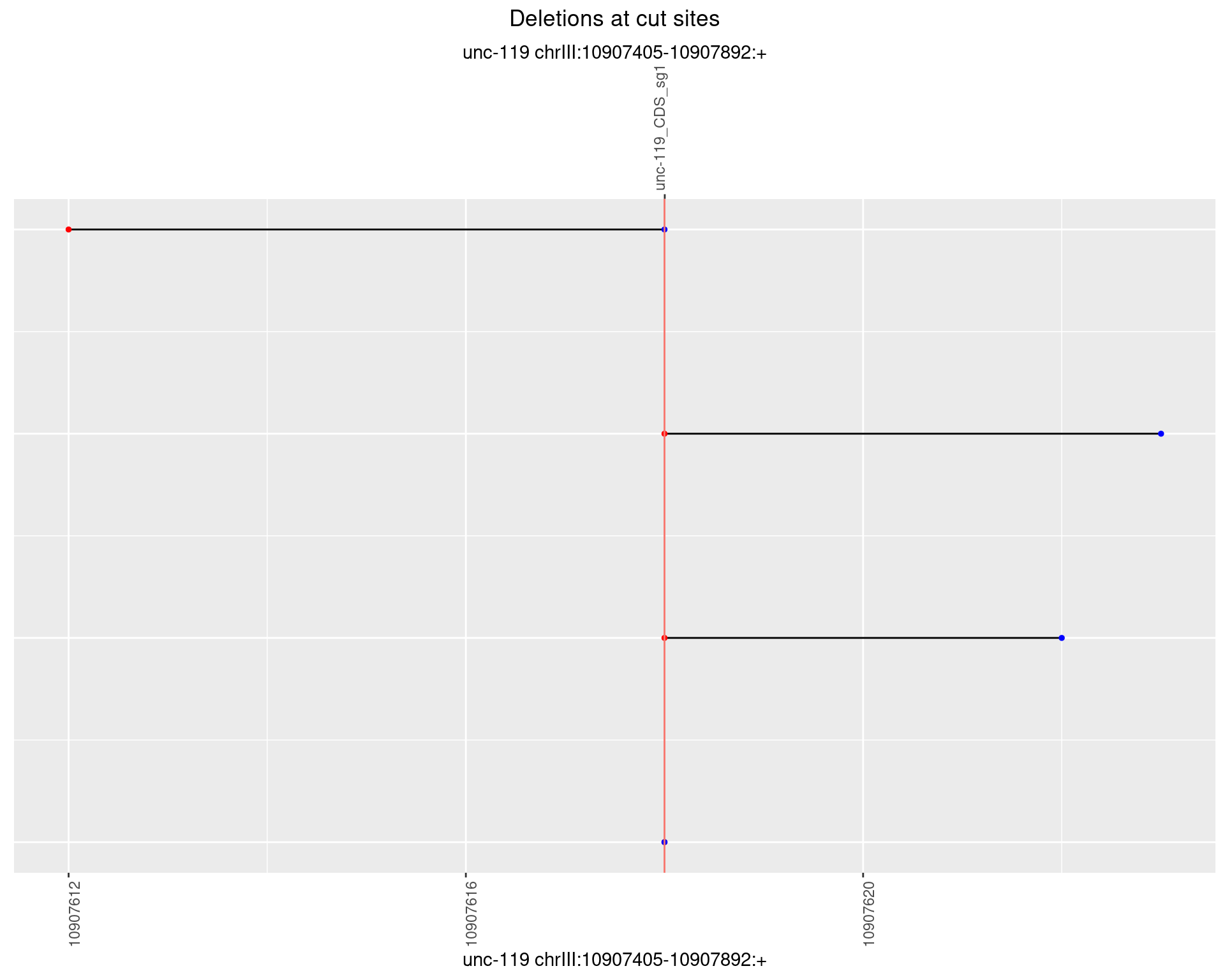
plotSegments <- function(dt, cs, readSupportThreshold = 0, freqThreshold = 0) {
dt <- dt[ReadSupport >= readSupportThreshold & freq >= freqThreshold]
if(nrow(dt) == 0){
return(NULL)
}
#first randomize the order (to avoid sorting by start position)
dt <- dt[sample(1:nrow(dt), nrow(dt))]
dt <- dt[order(end - start)]
dt$linePos <- 1:nrow(dt)
ggplot2::ggplot(dt, aes(x = linePos, ymin = start, ymax = end)) +
geom_linerange(size = 0.5) +
labs(title = "Deletions at cut sites") +
geom_point(data = dt, aes(x = linePos, y = start), size = 1, color = 'red') +
geom_point(data = dt, aes(x = linePos, y = end), size = 1, color = 'blue') +
geom_hline(data = cs,
aes(yintercept = start, color = name), show.legend = FALSE) +
theme(axis.text.y = element_blank(),
axis.title.y = element_blank(),
axis.ticks.y = element_blank(),
axis.text.x = element_text(angle = 90),
plot.title = element_text(hjust = 0.5)) +
scale_y_continuous(sec.axis = dup_axis(breaks = cs$start,
labels = cs$name)) +
coord_flip()
}
plots <- lapply(unique(deletionCutsiteOverlaps$sample), function(s) {
dt <- deletionCutsiteOverlaps[sample == s]
if(nrow(dt) == 0) {
return(NULL)
}
#segment plots with varying frequency thresholds
freqThresholds <- c(0, 0.00001, 0.0001, 0.001, 0.01, 0.1)
plots <- lapply(freqThresholds, function(t) {
p <- plotSegments(dt = dt[atCutSite == TRUE], #only plot those at cut sites
cs = as.data.frame(cutSites[cutSites$name %in% sampleGuides[[s]]]),
freqThreshold = t)
if(!is.null(p)) {
p <- p + labs(y = paste(targetName, targetRegion))
}
return(p)
})
names(plots) <- freqThresholds
return(plots)
})
names(plots) <- unique(deletionCutsiteOverlaps$sample)1 Deletion diversity at cut sites
# folder to save pdf versions of the segment plots
dirPath <- paste(targetName, 'Indel_Diversity.deletion_segment_plots', sep = '.')
if(!dir.exists(dirPath)) {
  dir.create(dirPath)
}
for (sample in names(plots)) {
  cat('## ',sample,'{.tabset .tabset-fade .tabset-pills}\n\n')
  for(i in names(plots[[sample]])) {
    cat('### Freq:',i,'\n\n')
    p <- plots[[sample]][[i]]
    if(!is.null(p)) {
      print(p)
      ggsave(filename = file.path(dirPath, paste(sample, 'freq', i, 'pdf', sep = '.')),
             plot = p, width = 10, height = 8, units = 'in')
    } else {
      cat("No plot to show\n\n")
    }
    cat("\n\n")
  }
  cat("\n\n")
}
1.1 gen_24C_F2_unc-119_N2
1.1.1 Freq: 0
1.1.2 Freq: 1e-05
1.1.3 Freq: 1e-04
1.1.4 Freq: 0.001
No plot to show
1.1.5 Freq: 0.01
No plot to show
1.1.6 Freq: 0.1
No plot to show
1.2 gen_24C_F2_unc-119_sg1
1.2.1 Freq: 0
1.2.2 Freq: 1e-05
1.2.3 Freq: 1e-04
1.2.4 Freq: 0.001
1.2.5 Freq: 0.01
No plot to show
1.2.6 Freq: 0.1
No plot to show
1.3 gen_24C_F3_unc-119_N2
1.3.1 Freq: 0
1.3.2 Freq: 1e-05
1.3.3 Freq: 1e-04

1.3.4 Freq: 0.001
No plot to show
1.3.5 Freq: 0.01
No plot to show
1.3.6 Freq: 0.1
No plot to show
1.4 gen_24C_F3_unc-119_sg1
1.4.1 Freq: 0
1.4.2 Freq: 1e-05
1.4.3 Freq: 1e-04
1.4.4 Freq: 0.001

1.4.5 Freq: 0.01
No plot to show
1.4.6 Freq: 0.1
No plot to show
1.5 gen_24C_F4_unc-119_N2
1.5.1 Freq: 0
1.5.2 Freq: 1e-05
1.5.3 Freq: 1e-04

1.5.4 Freq: 0.001
No plot to show
1.5.5 Freq: 0.01
No plot to show
1.5.6 Freq: 0.1
No plot to show
1.6 gen_24C_F4_unc-119_sg1
1.6.1 Freq: 0
1.6.2 Freq: 1e-05
1.6.3 Freq: 1e-04
1.6.4 Freq: 0.001

1.6.5 Freq: 0.01
No plot to show
1.6.6 Freq: 0.1
No plot to show
1.7 gen_24C_F5_unc-119_N2
1.7.1 Freq: 0
1.7.2 Freq: 1e-05
1.7.3 Freq: 1e-04

1.7.4 Freq: 0.001
No plot to show
1.7.5 Freq: 0.01
No plot to show
1.7.6 Freq: 0.1
No plot to show
1.8 gen_24C_F5_unc-119_sg1
1.8.1 Freq: 0
1.8.2 Freq: 1e-05
1.8.3 Freq: 1e-04
1.8.4 Freq: 0.001

1.8.5 Freq: 0.01
No plot to show
1.8.6 Freq: 0.1
No plot to show
1.9 gen_16C_F2_unc-119_N2
1.9.1 Freq: 0
1.9.2 Freq: 1e-05
1.9.3 Freq: 1e-04

1.9.4 Freq: 0.001
No plot to show
1.9.5 Freq: 0.01
No plot to show
1.9.6 Freq: 0.1
No plot to show
1.10 gen_16C_F2_unc-119_sg1
1.10.1 Freq: 0
1.10.2 Freq: 1e-05
1.10.3 Freq: 1e-04
1.10.4 Freq: 0.001
1.10.5 Freq: 0.01
No plot to show
1.10.6 Freq: 0.1
No plot to show
1.11 gen_16C_F3_unc-119_N2
1.11.1 Freq: 0
1.11.2 Freq: 1e-05
1.11.3 Freq: 1e-04

1.11.4 Freq: 0.001
No plot to show
1.11.5 Freq: 0.01
No plot to show
1.11.6 Freq: 0.1
No plot to show
1.12 gen_16C_F3_unc-119_sg1
1.12.1 Freq: 0
1.12.2 Freq: 1e-05
1.12.3 Freq: 1e-04

1.12.4 Freq: 0.001

1.12.5 Freq: 0.01
No plot to show
1.12.6 Freq: 0.1
No plot to show
1.13 gen_16C_F4_unc-119_N2
1.13.1 Freq: 0
1.13.2 Freq: 1e-05
1.13.3 Freq: 1e-04
1.13.4 Freq: 0.001
No plot to show
1.13.5 Freq: 0.01
No plot to show
1.13.6 Freq: 0.1
No plot to show
1.14 gen_16C_F4_unc-119_sg1
1.14.1 Freq: 0

1.14.2 Freq: 1e-05
1.14.3 Freq: 1e-04
1.14.4 Freq: 0.001
1.14.5 Freq: 0.01
No plot to show
1.14.6 Freq: 0.1
No plot to show
1.15 gen_16C_F5_unc-119_N2
1.15.1 Freq: 0
1.15.2 Freq: 1e-05
1.15.3 Freq: 1e-04
1.15.4 Freq: 0.001
No plot to show
1.15.5 Freq: 0.01
No plot to show
1.15.6 Freq: 0.1
No plot to show
1.16 gen_16C_F5_unc-119_sg1
1.16.1 Freq: 0
1.16.2 Freq: 1e-05
1.16.3 Freq: 1e-04
1.16.4 Freq: 0.001
No plot to show
1.16.5 Freq: 0.01
No plot to show
1.16.6 Freq: 0.1
No plot to show
1.17 gen_1624C_F1_unc-119_N2
1.17.1 Freq: 0
1.17.2 Freq: 1e-05
1.17.3 Freq: 1e-04

1.17.4 Freq: 0.001
No plot to show
1.17.5 Freq: 0.01
No plot to show
1.17.6 Freq: 0.1
No plot to show
1.18 gen_1624C_F1_unc-119_sg1
1.18.1 Freq: 0
1.18.2 Freq: 1e-05
1.18.3 Freq: 1e-04
1.18.4 Freq: 0.001
1.18.5 Freq: 0.01
No plot to show
1.18.6 Freq: 0.1
No plot to show
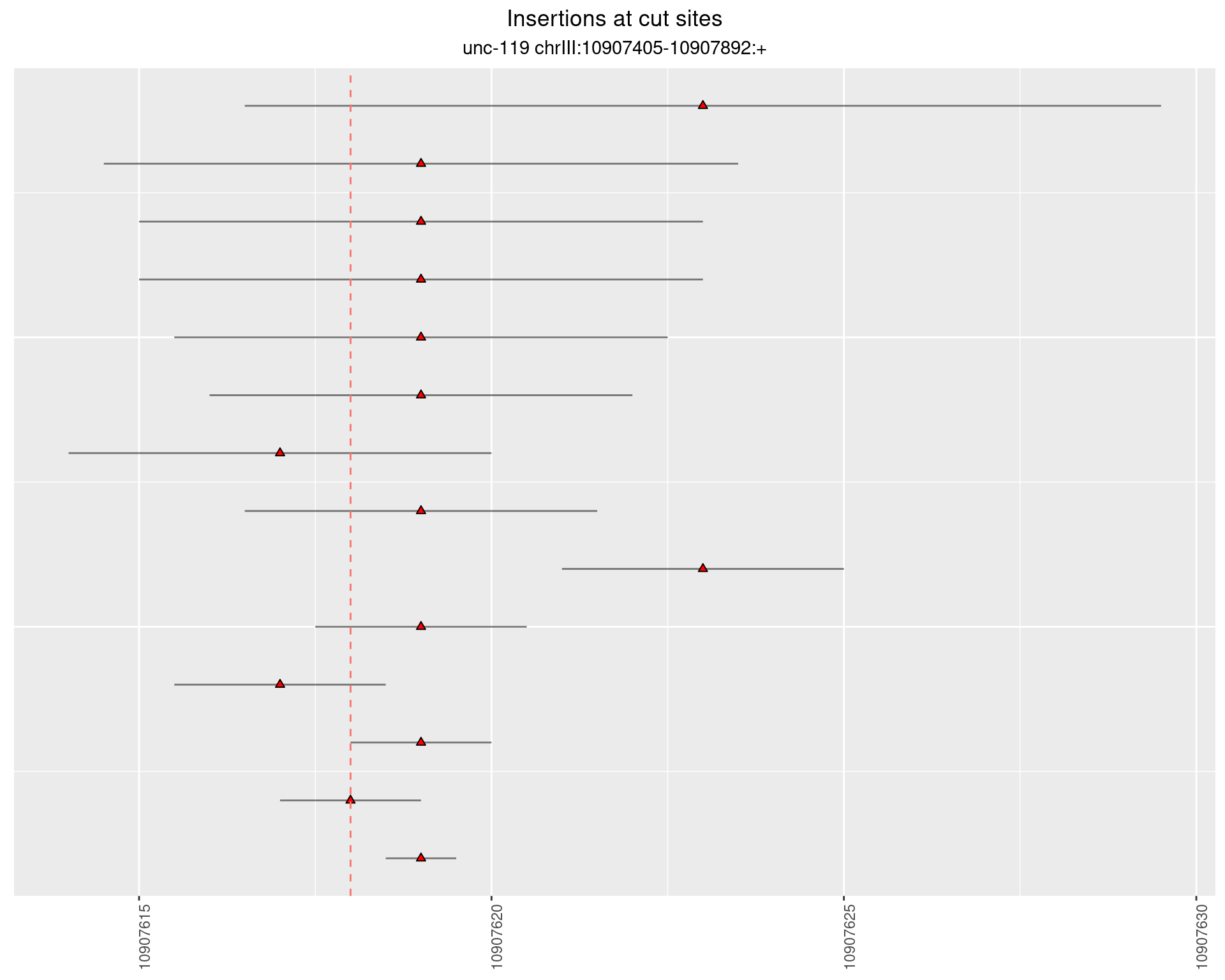
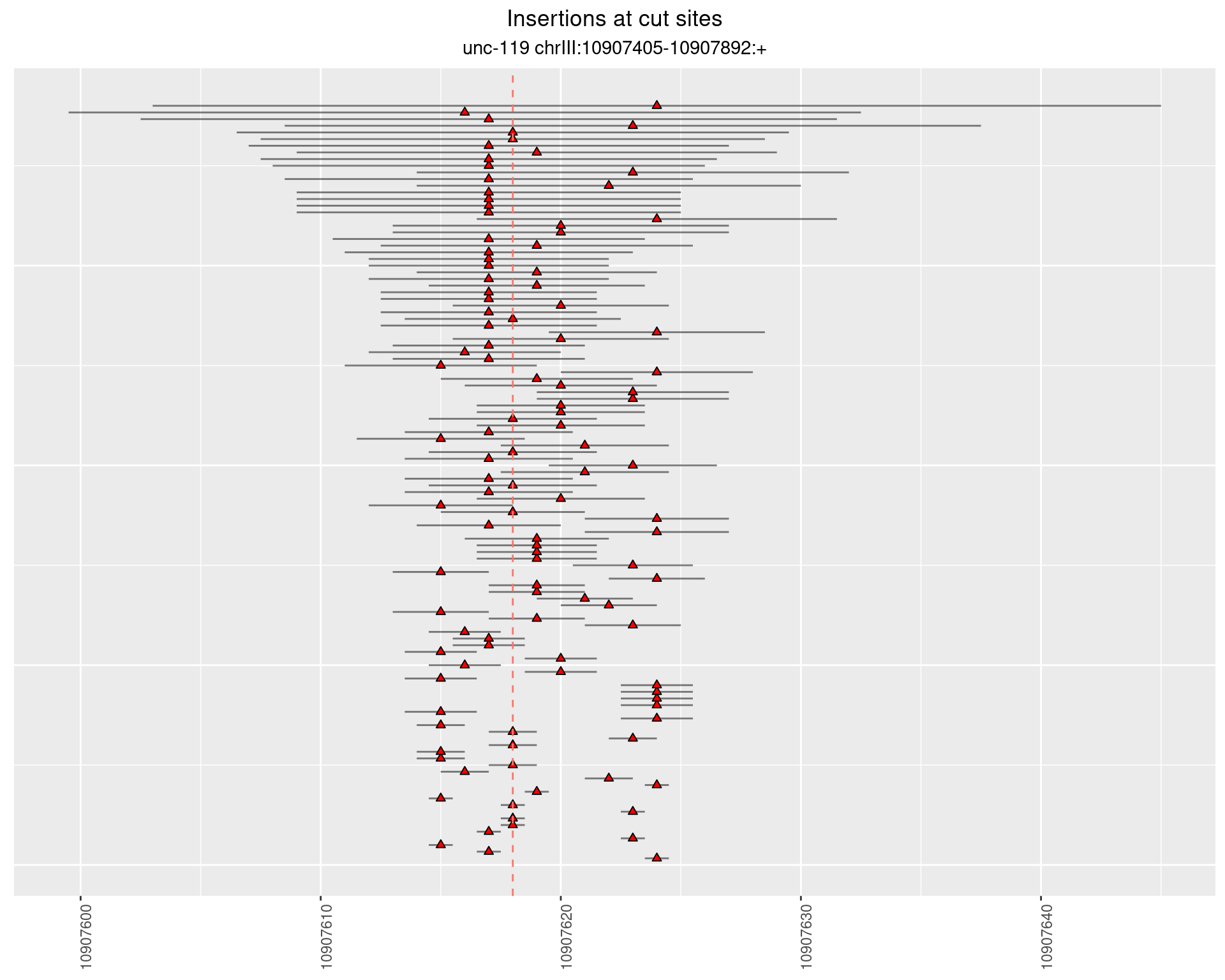
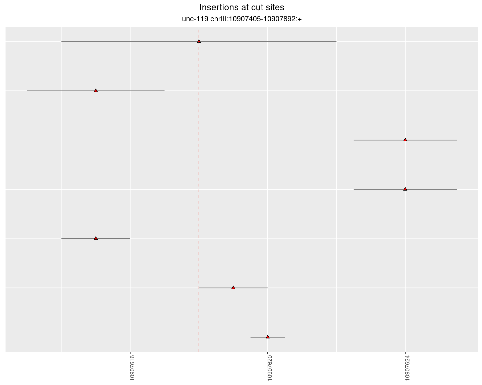
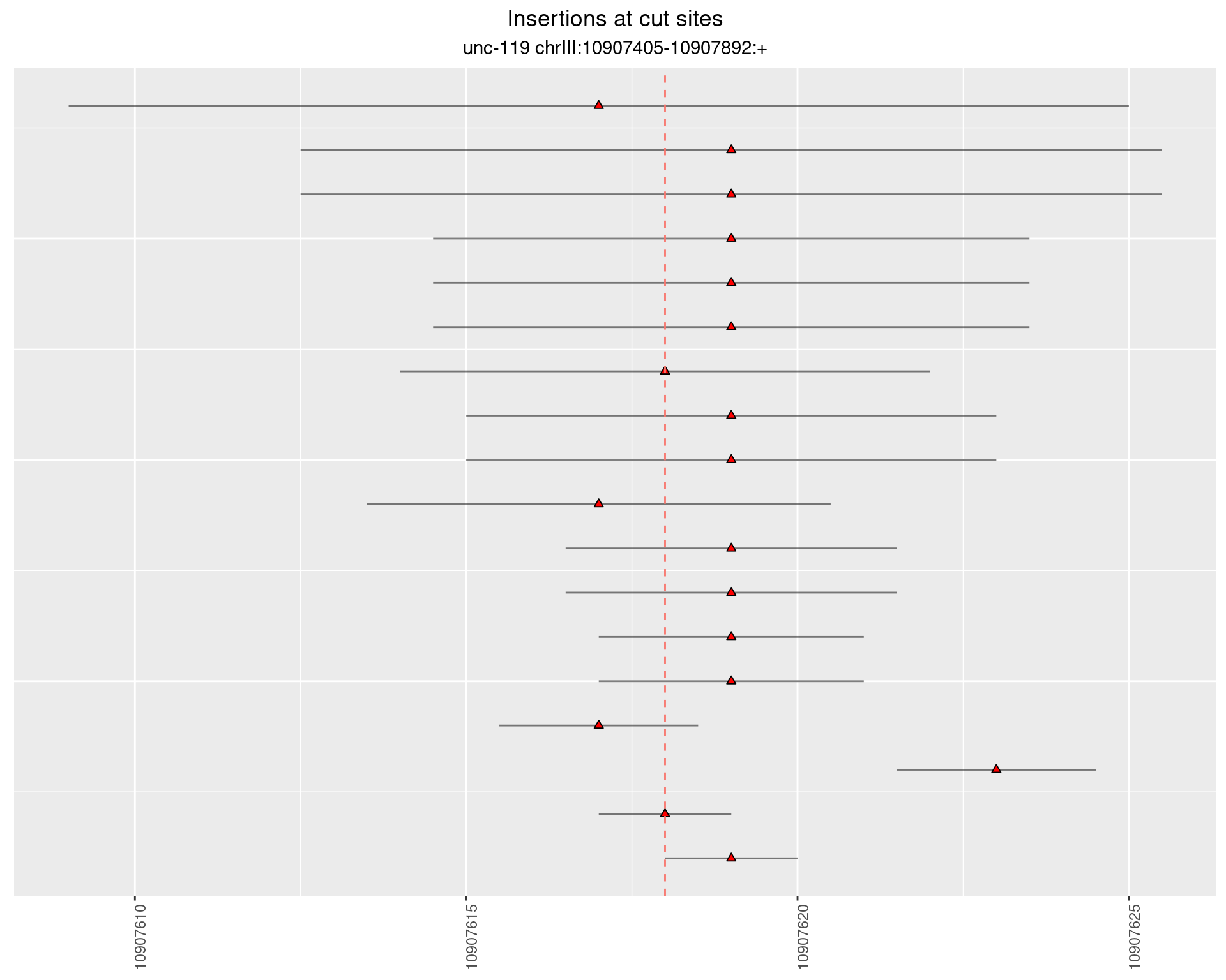
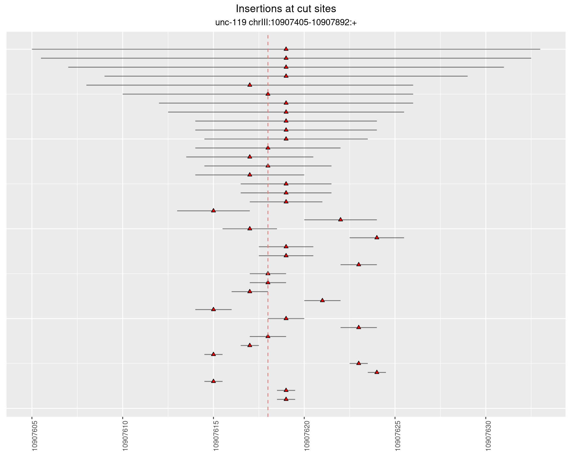
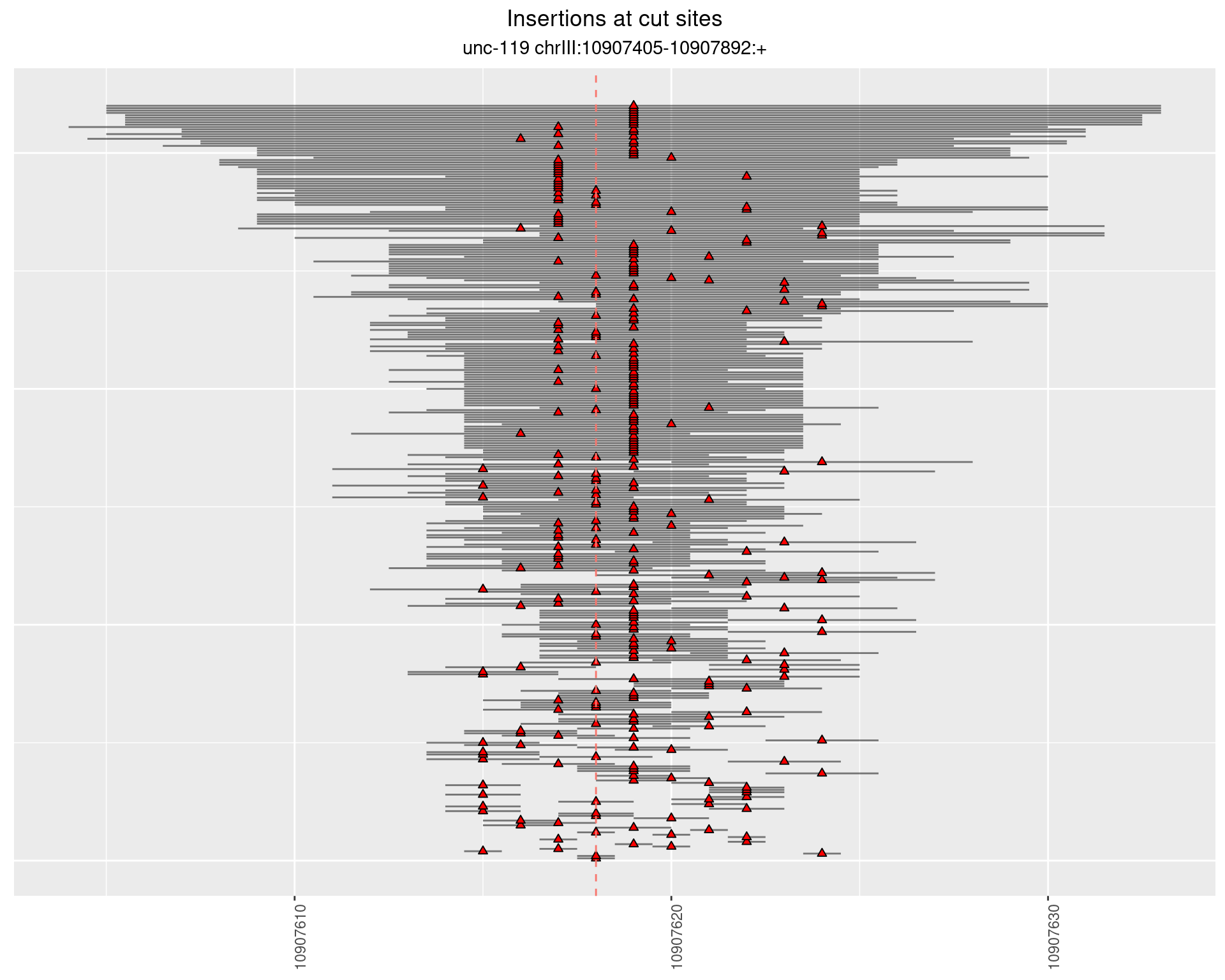
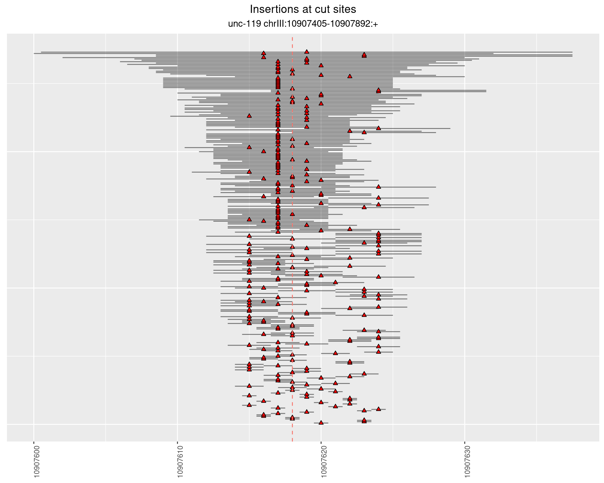
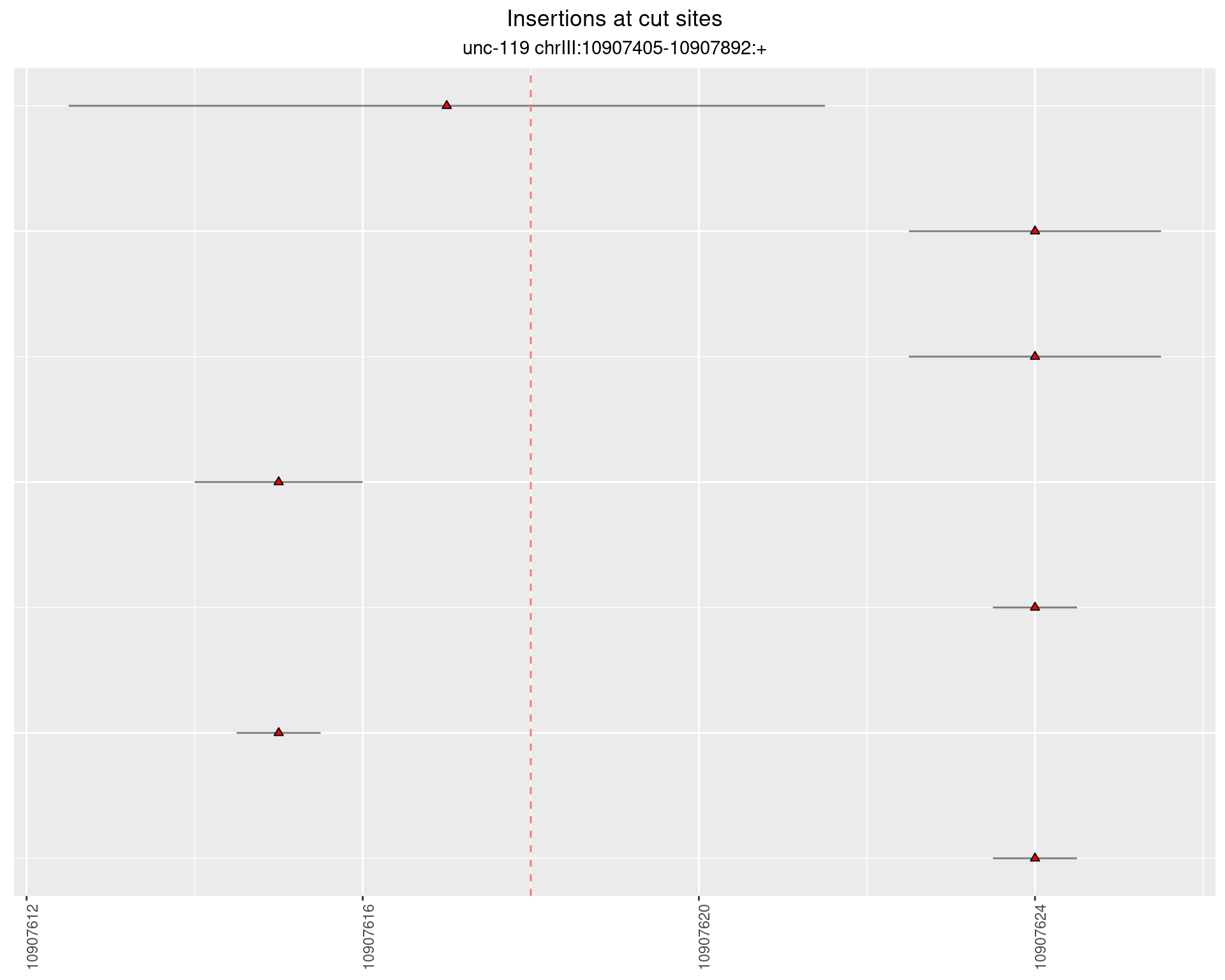
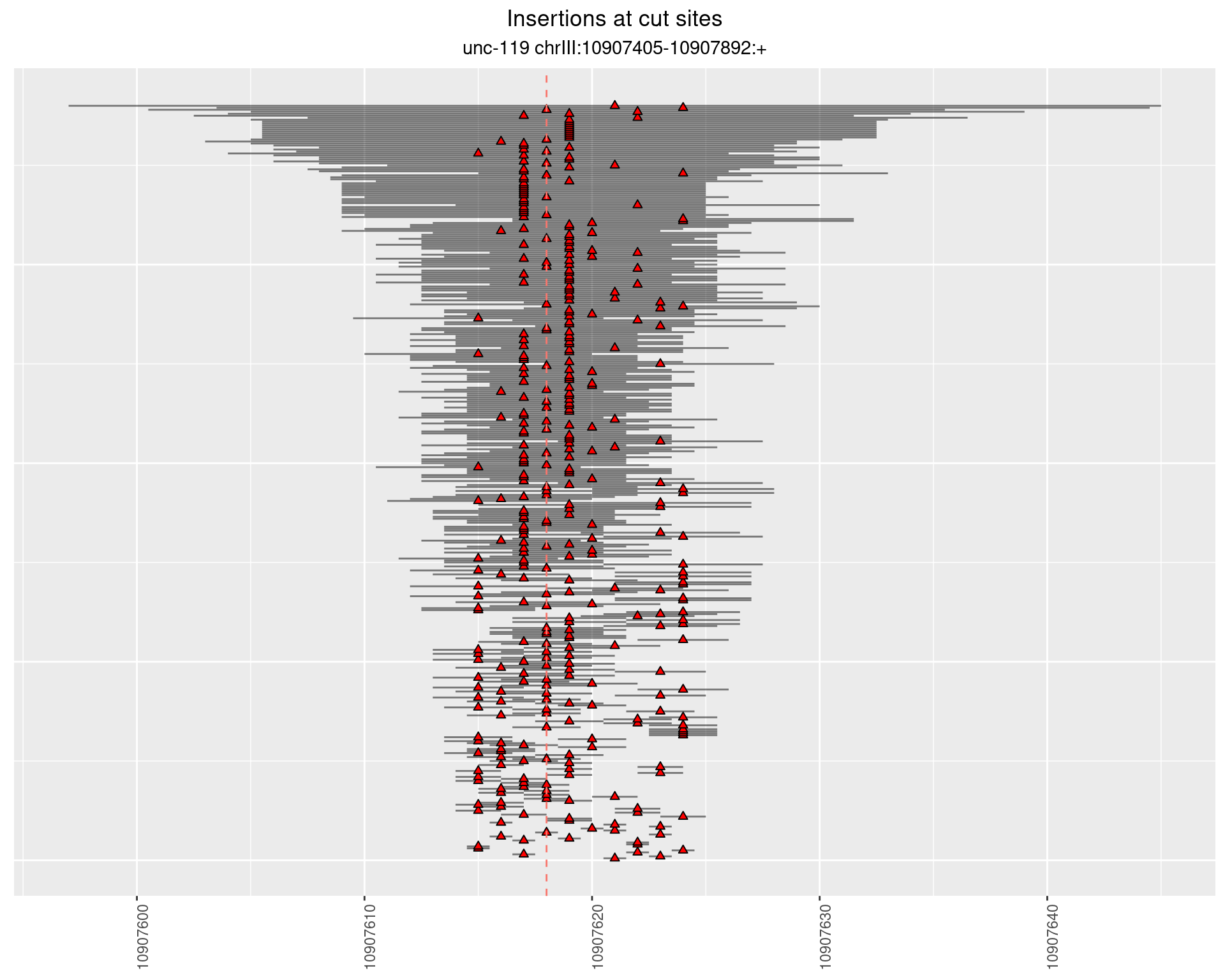
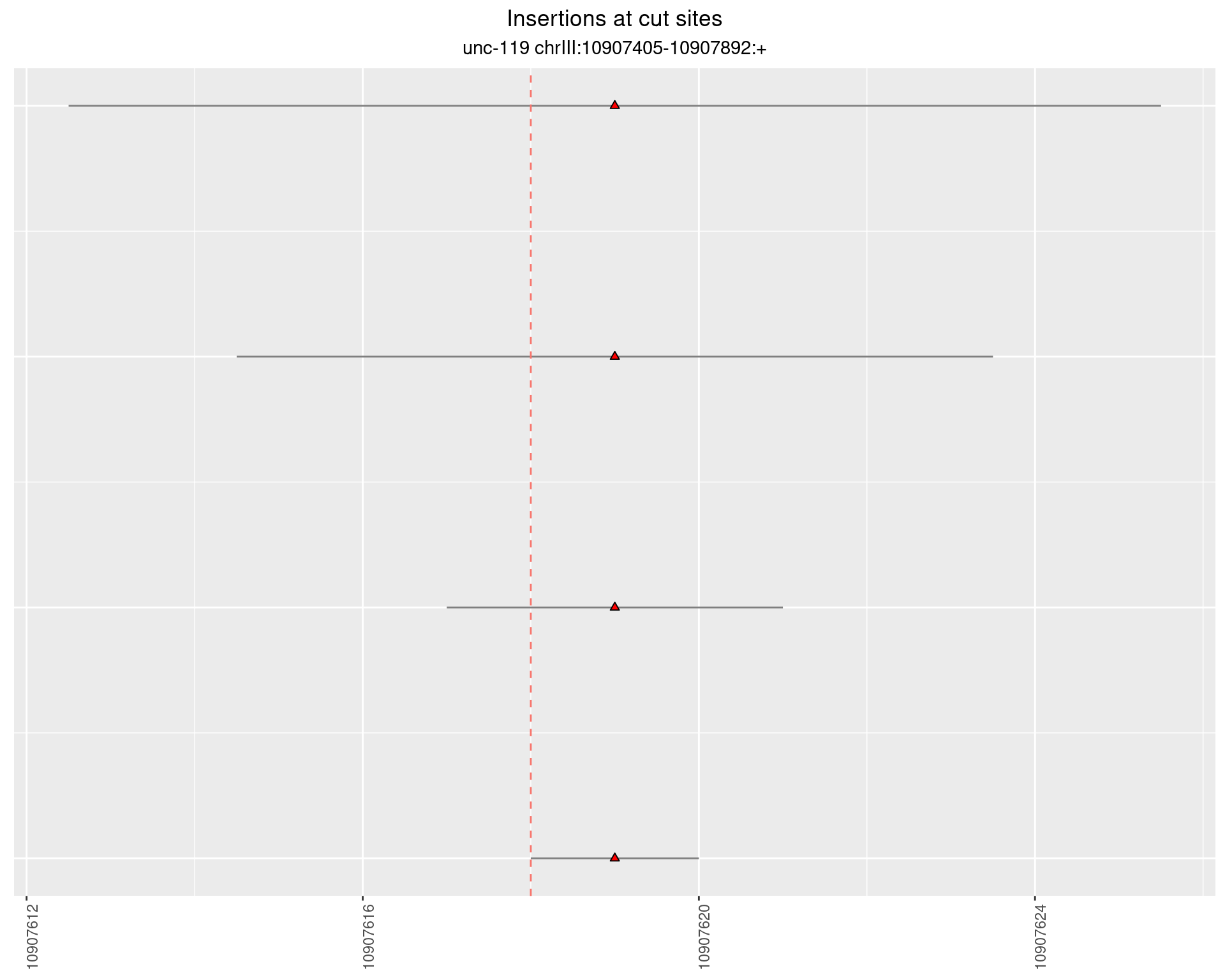
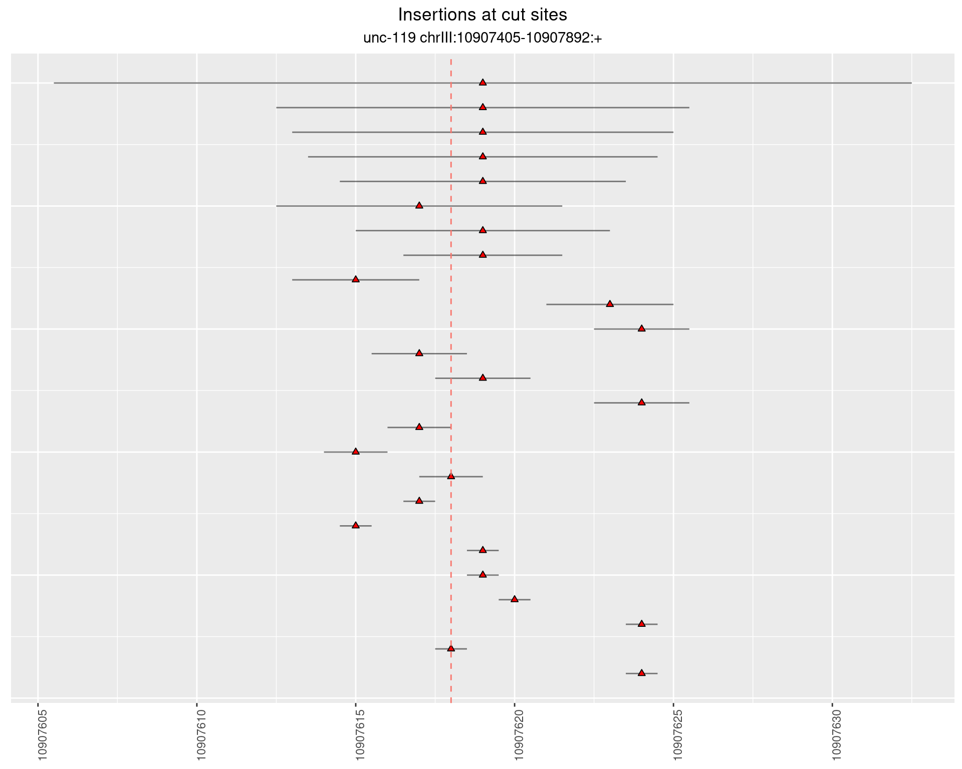
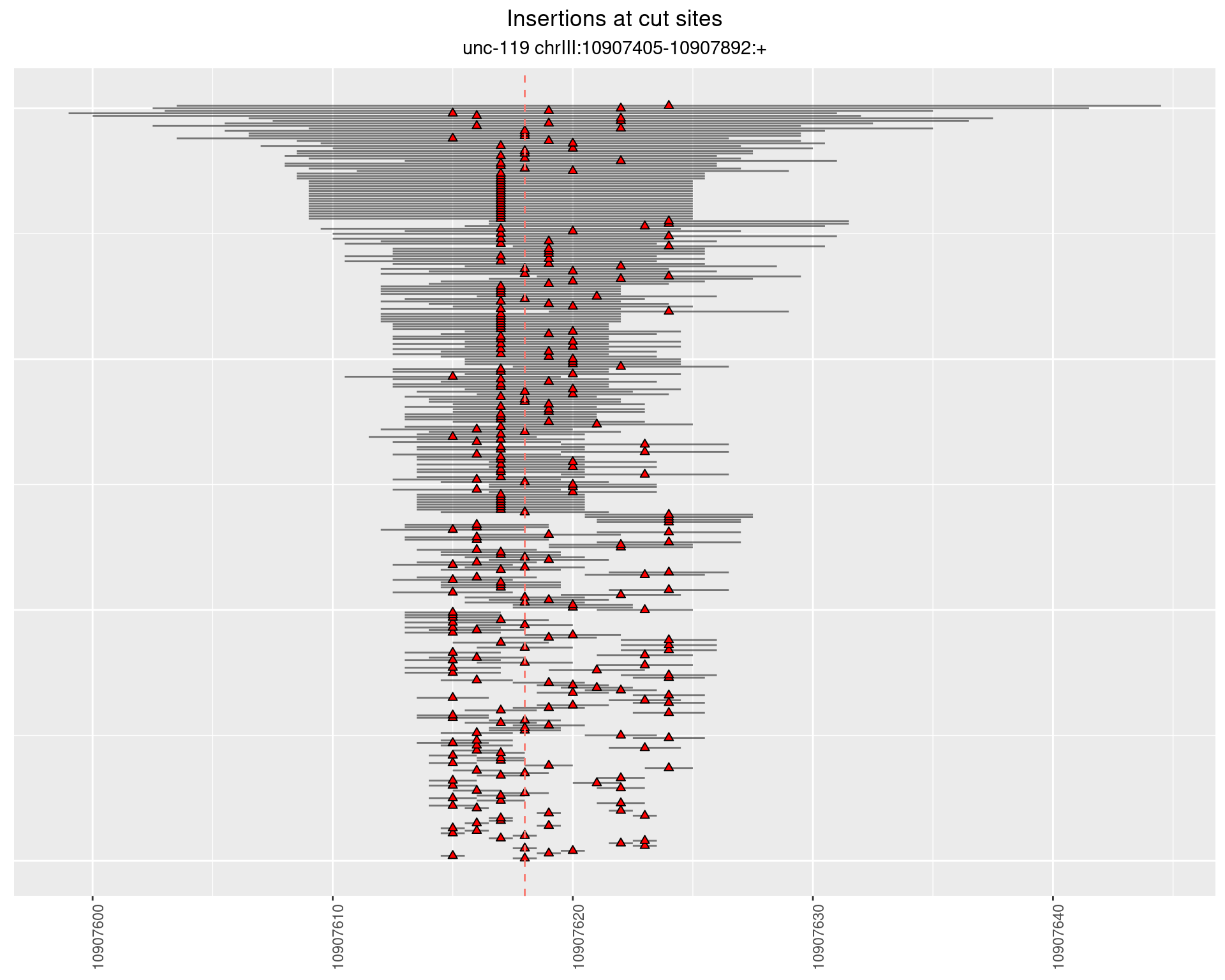
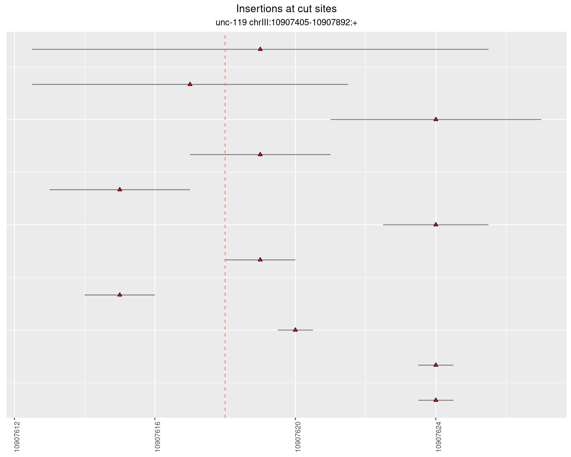
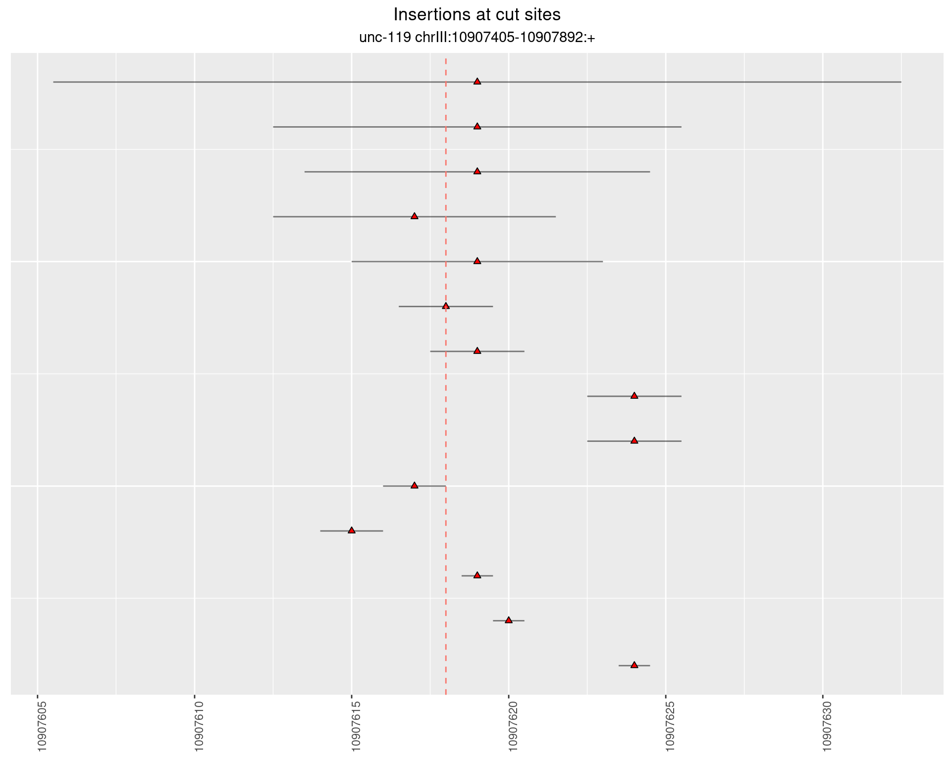
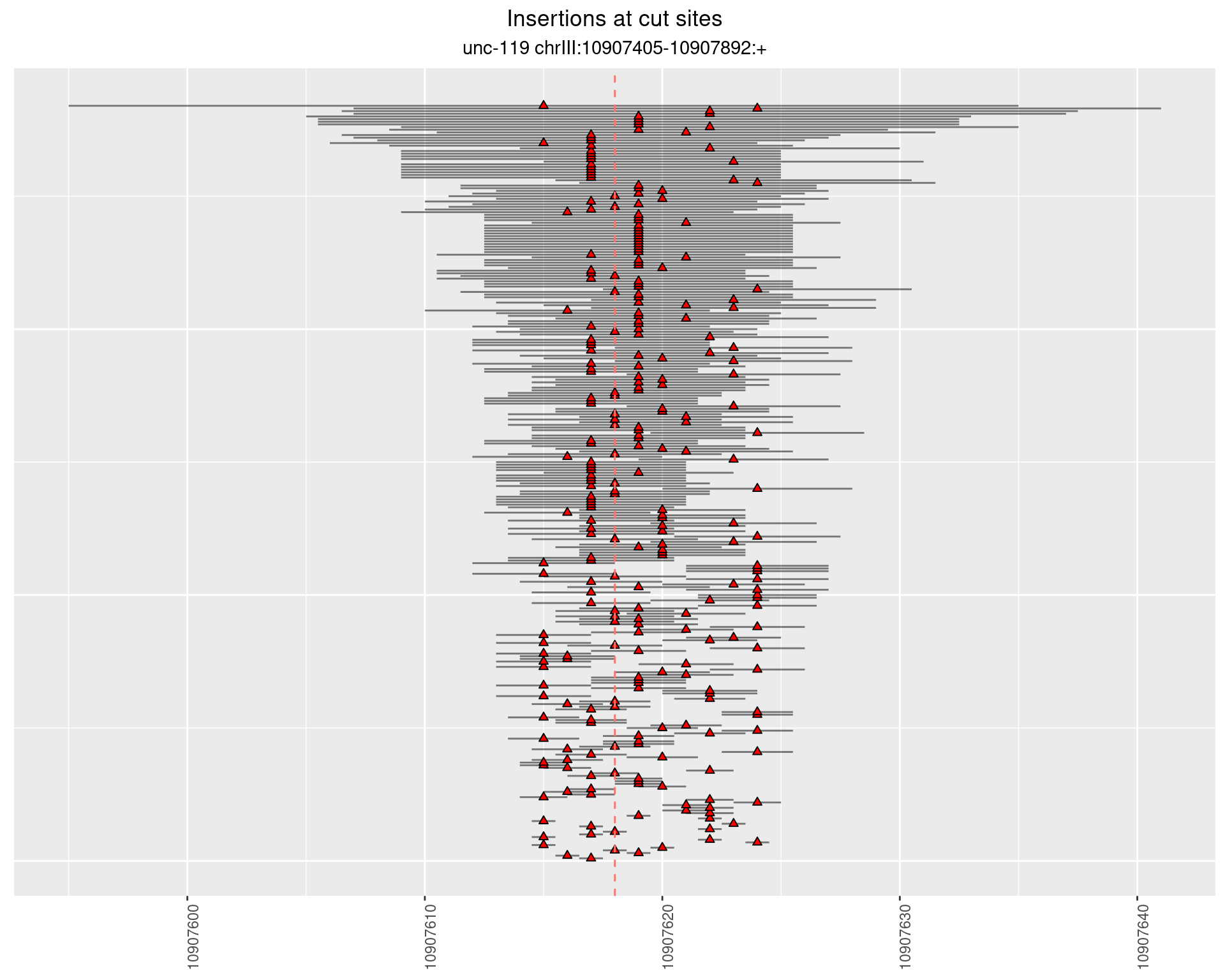
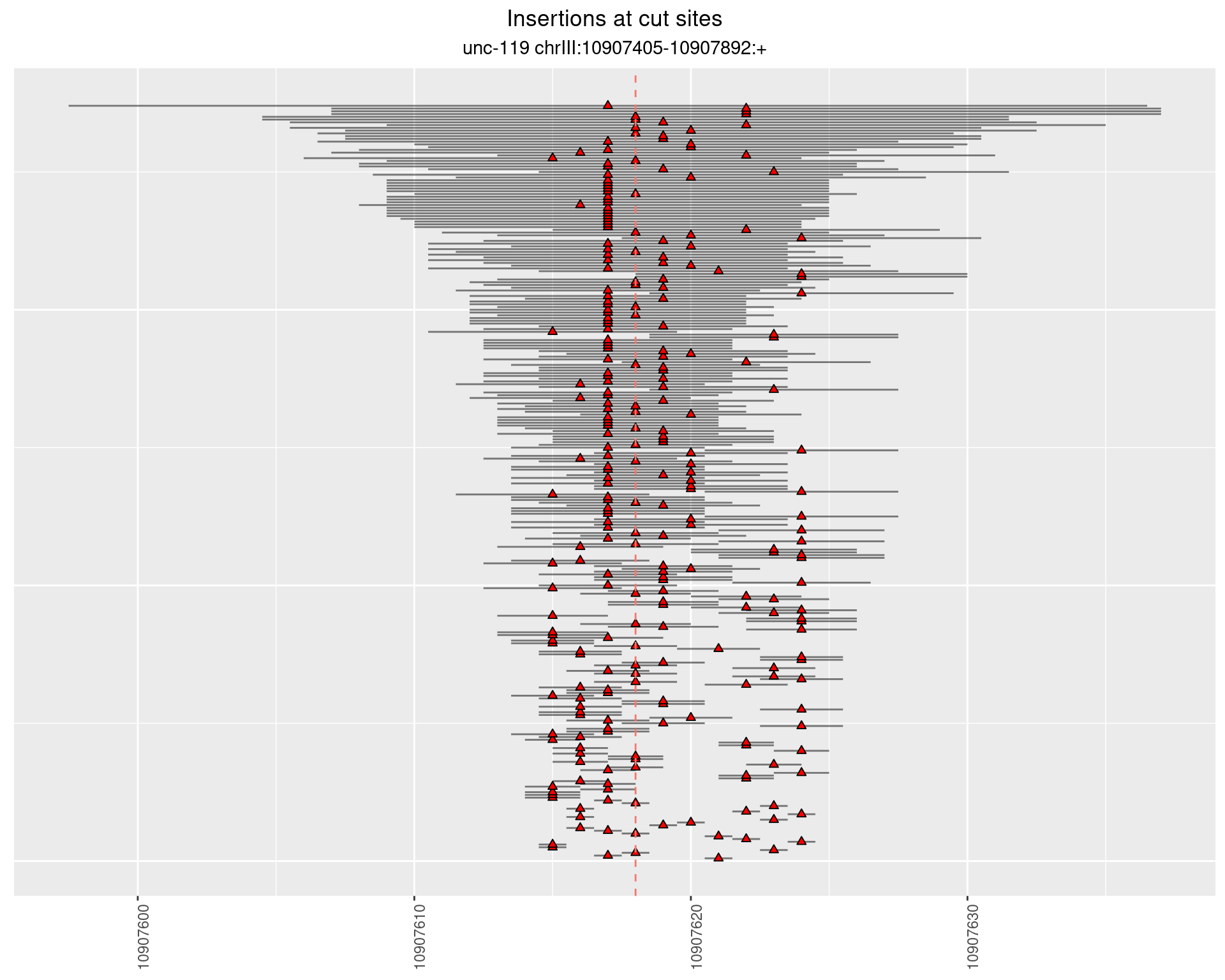
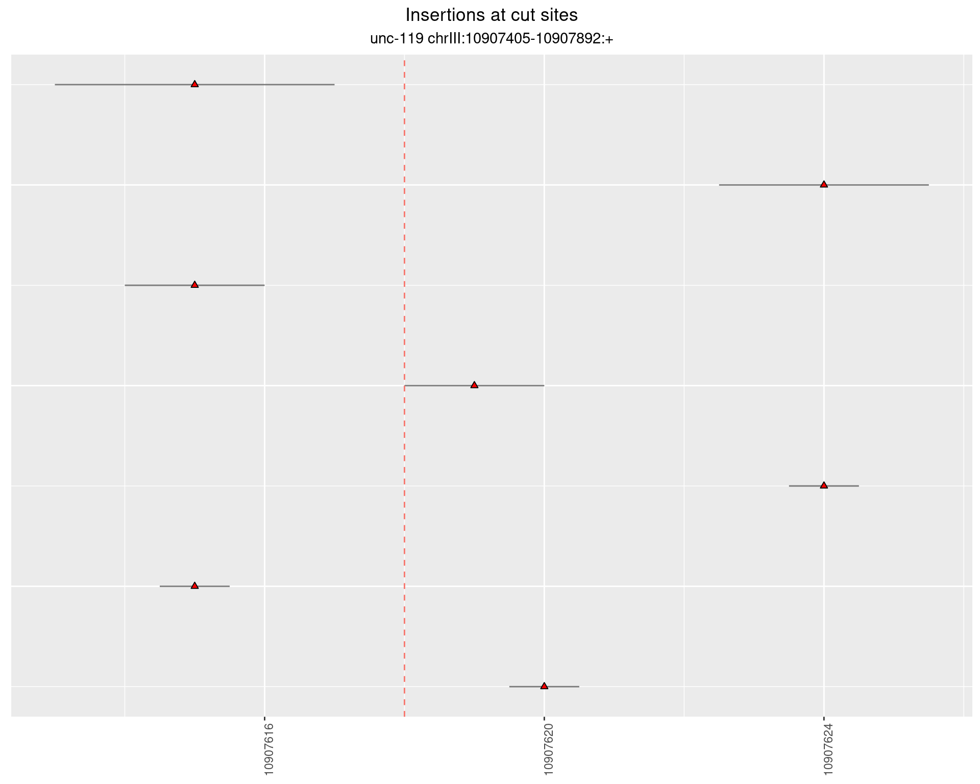
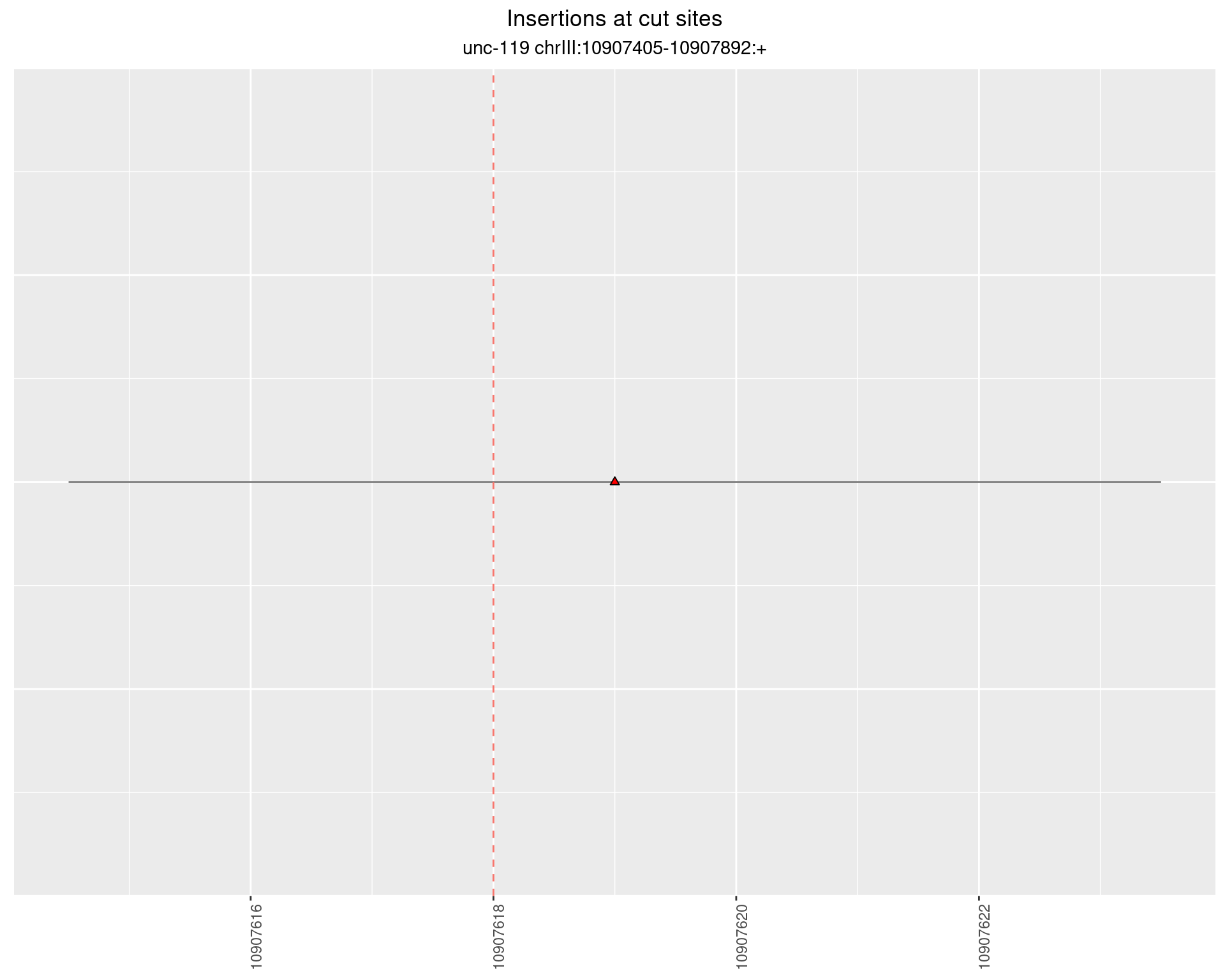
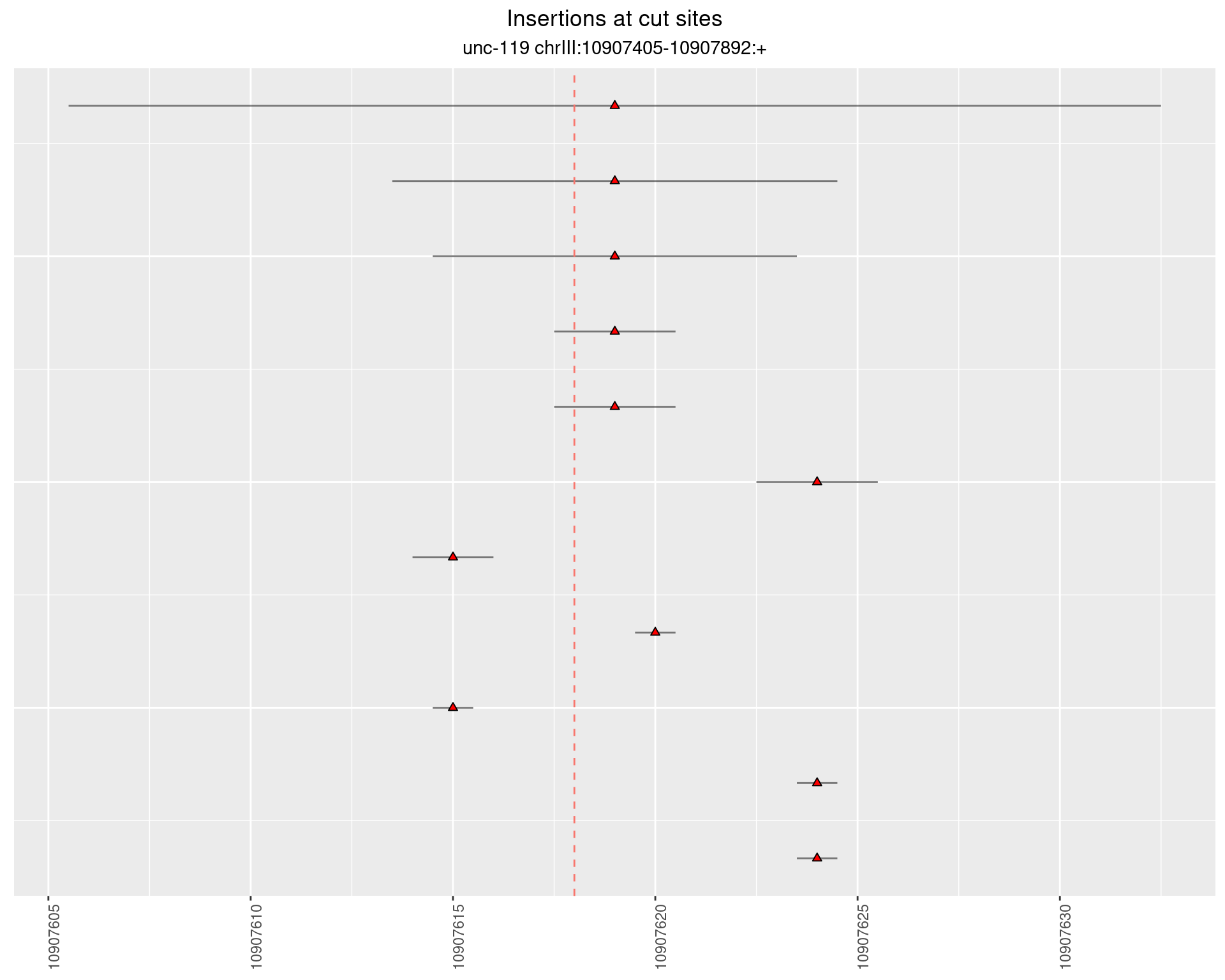
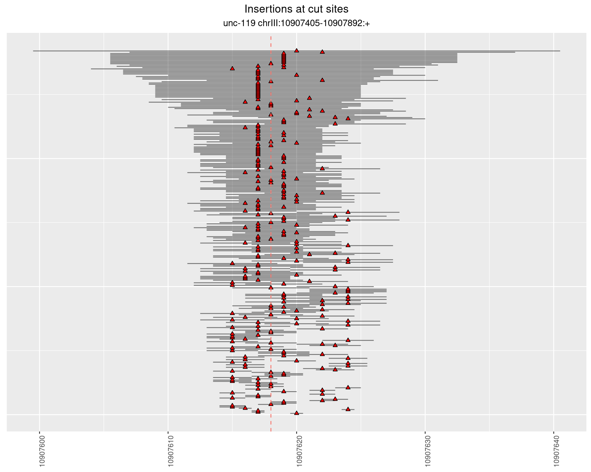
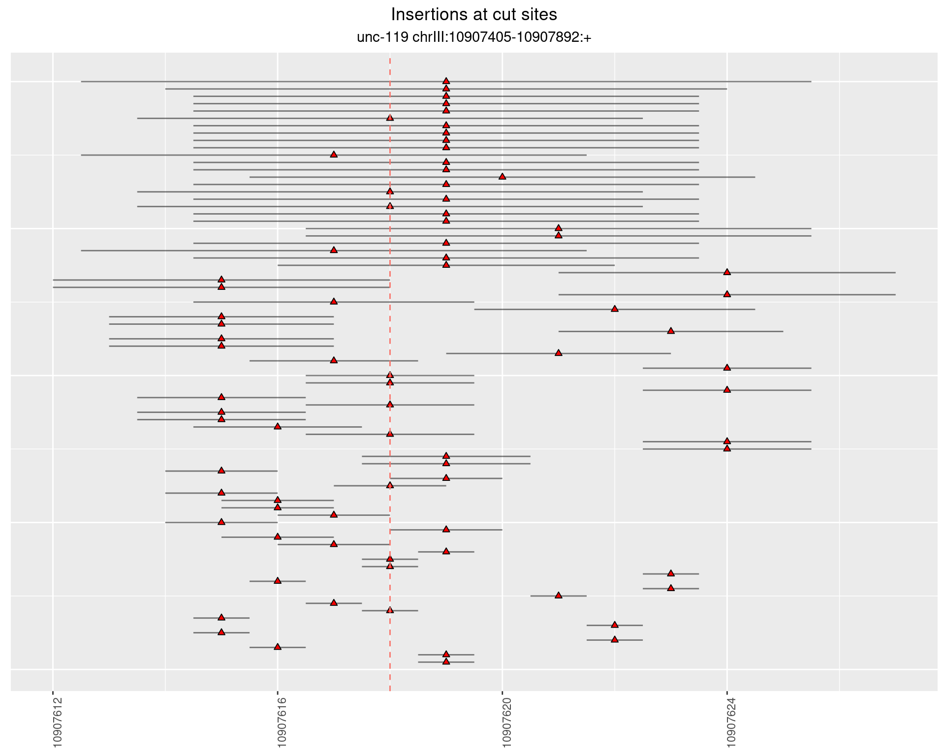
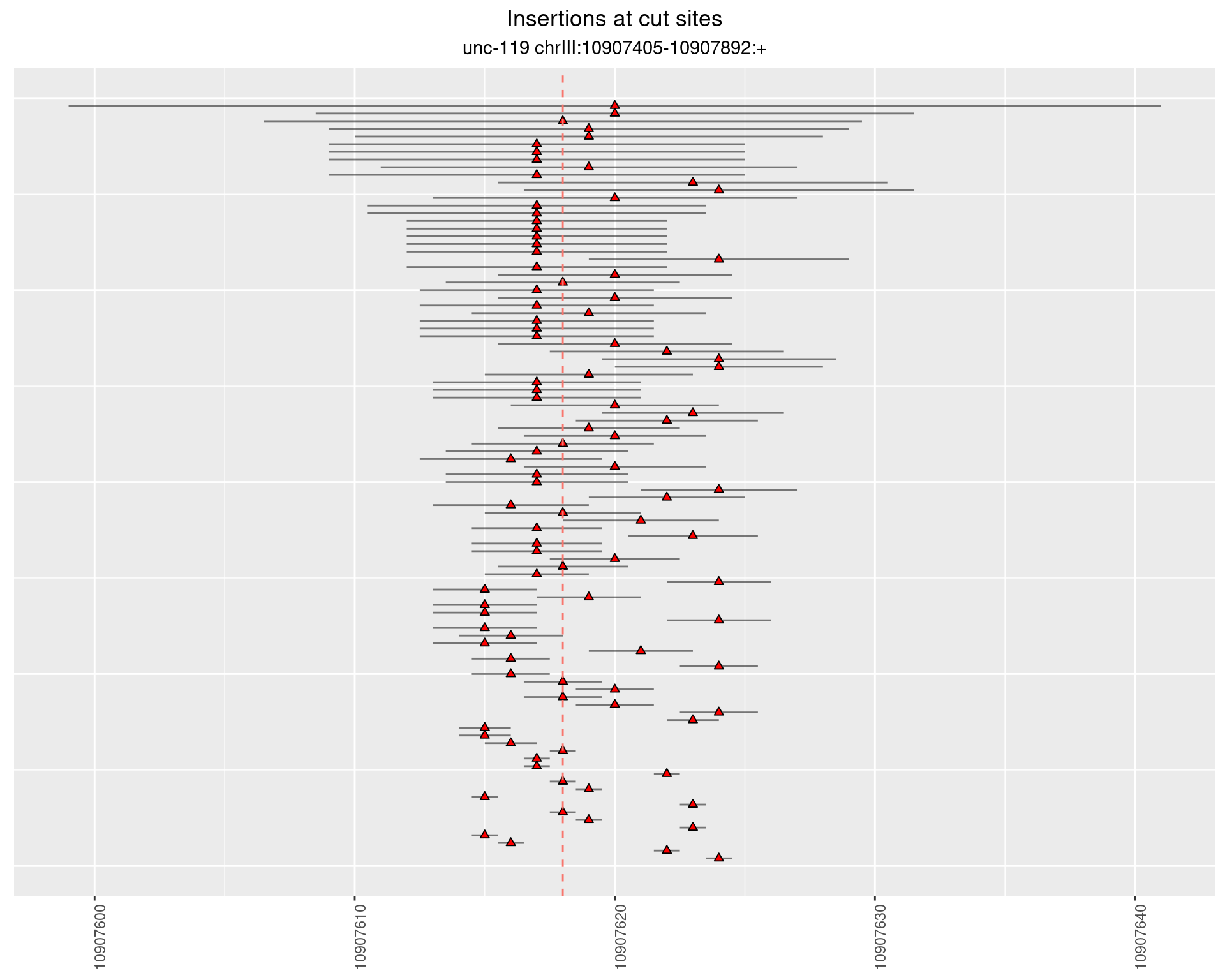
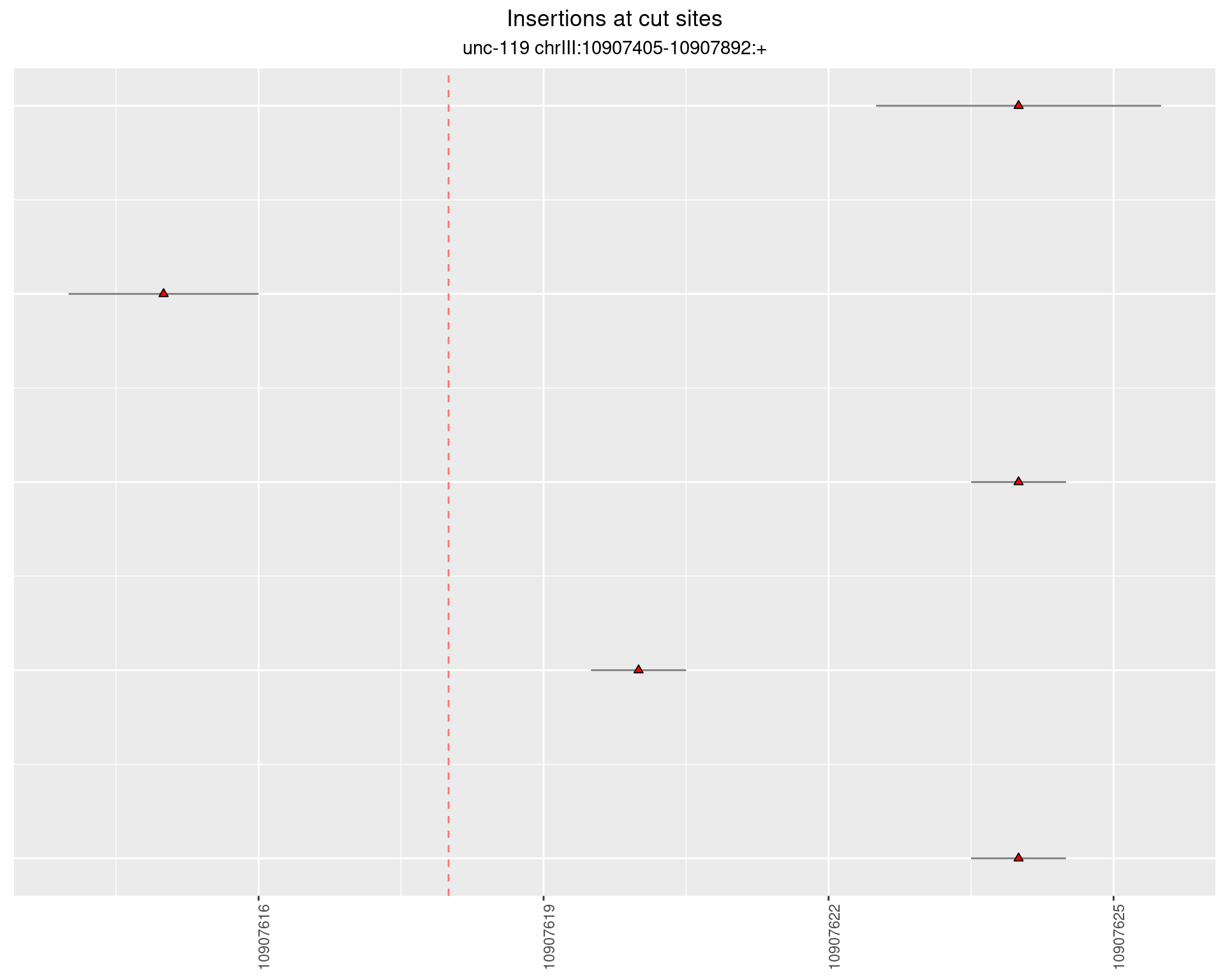
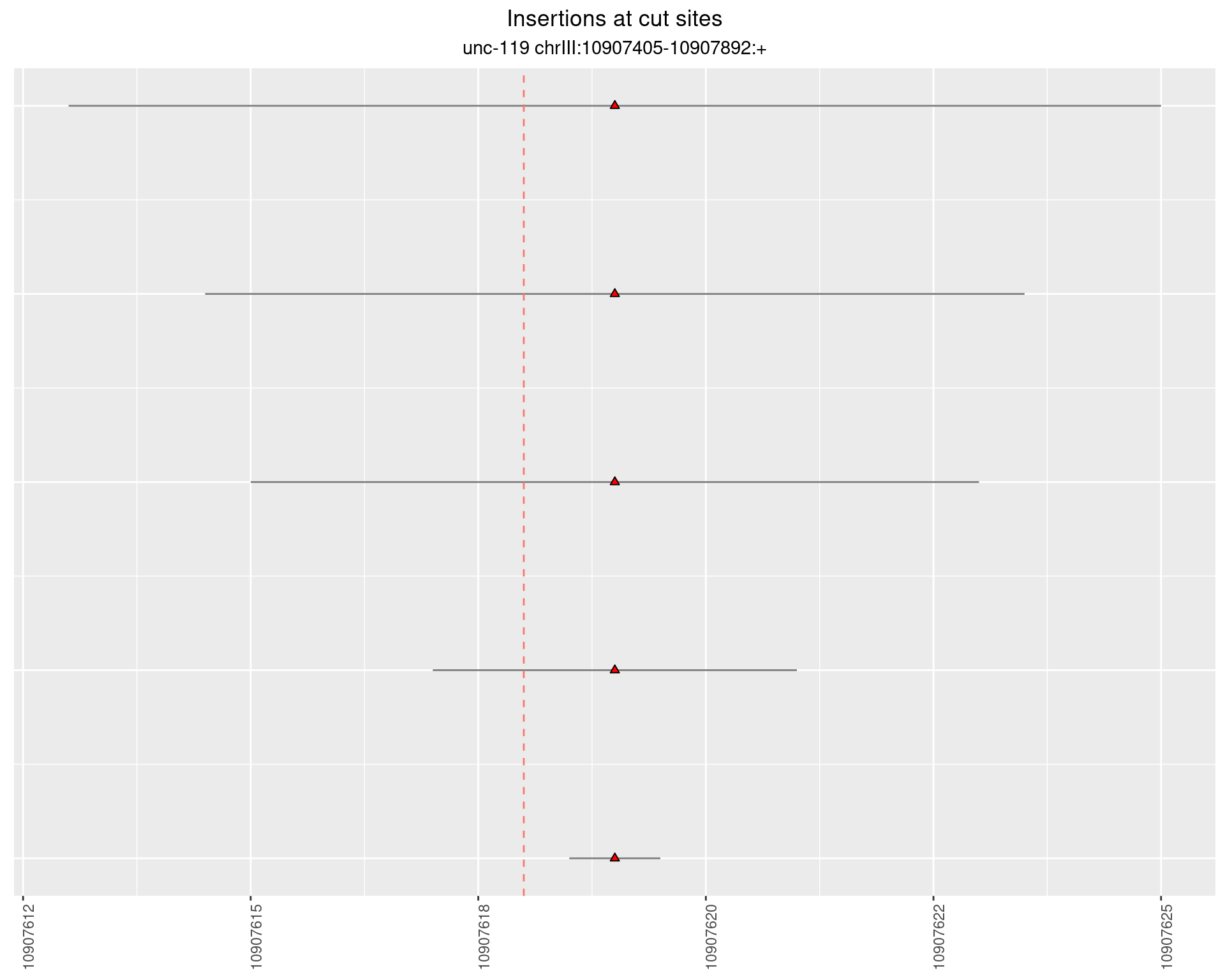
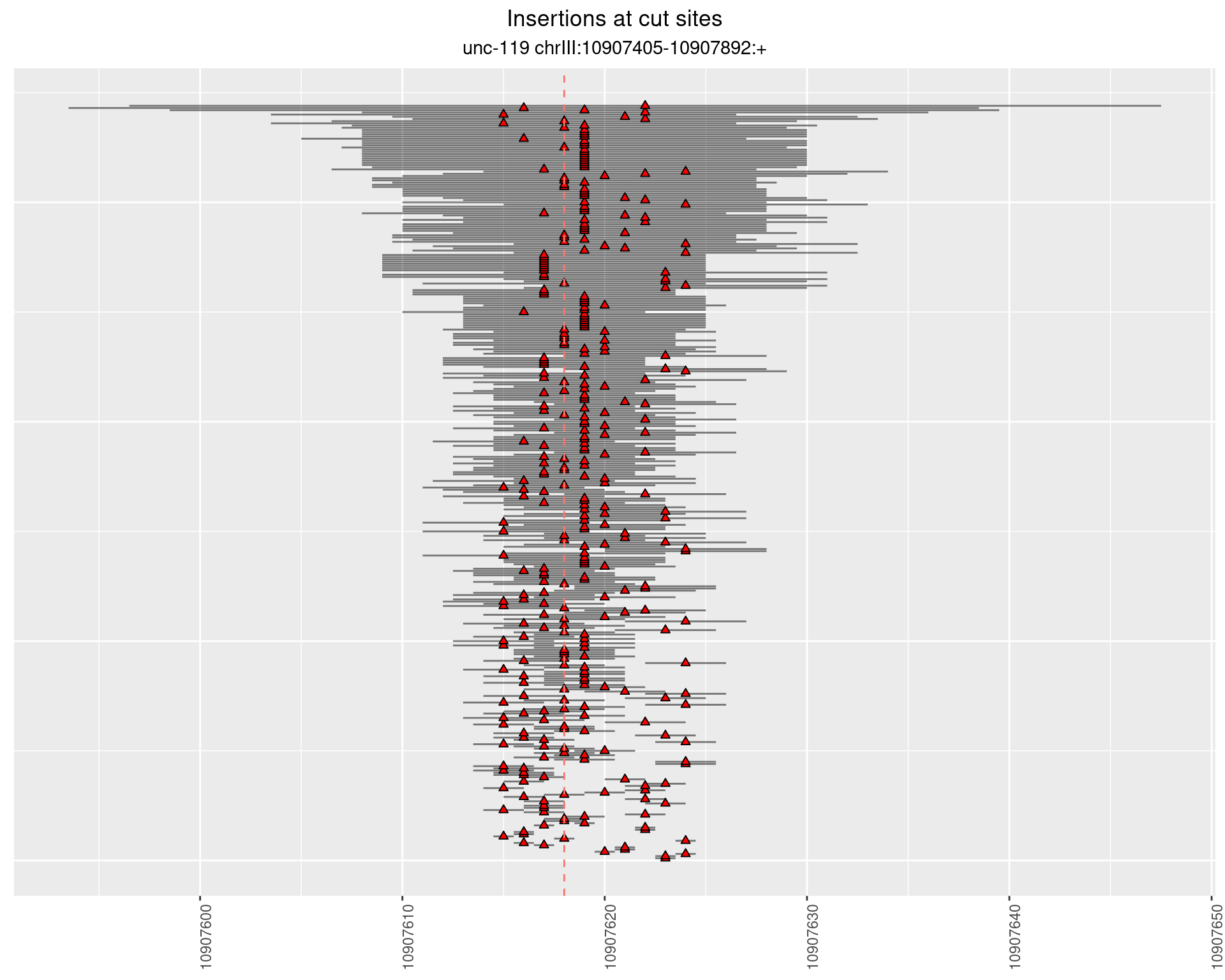
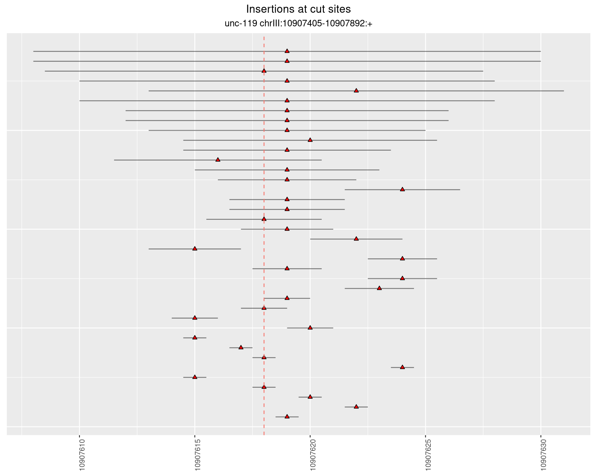
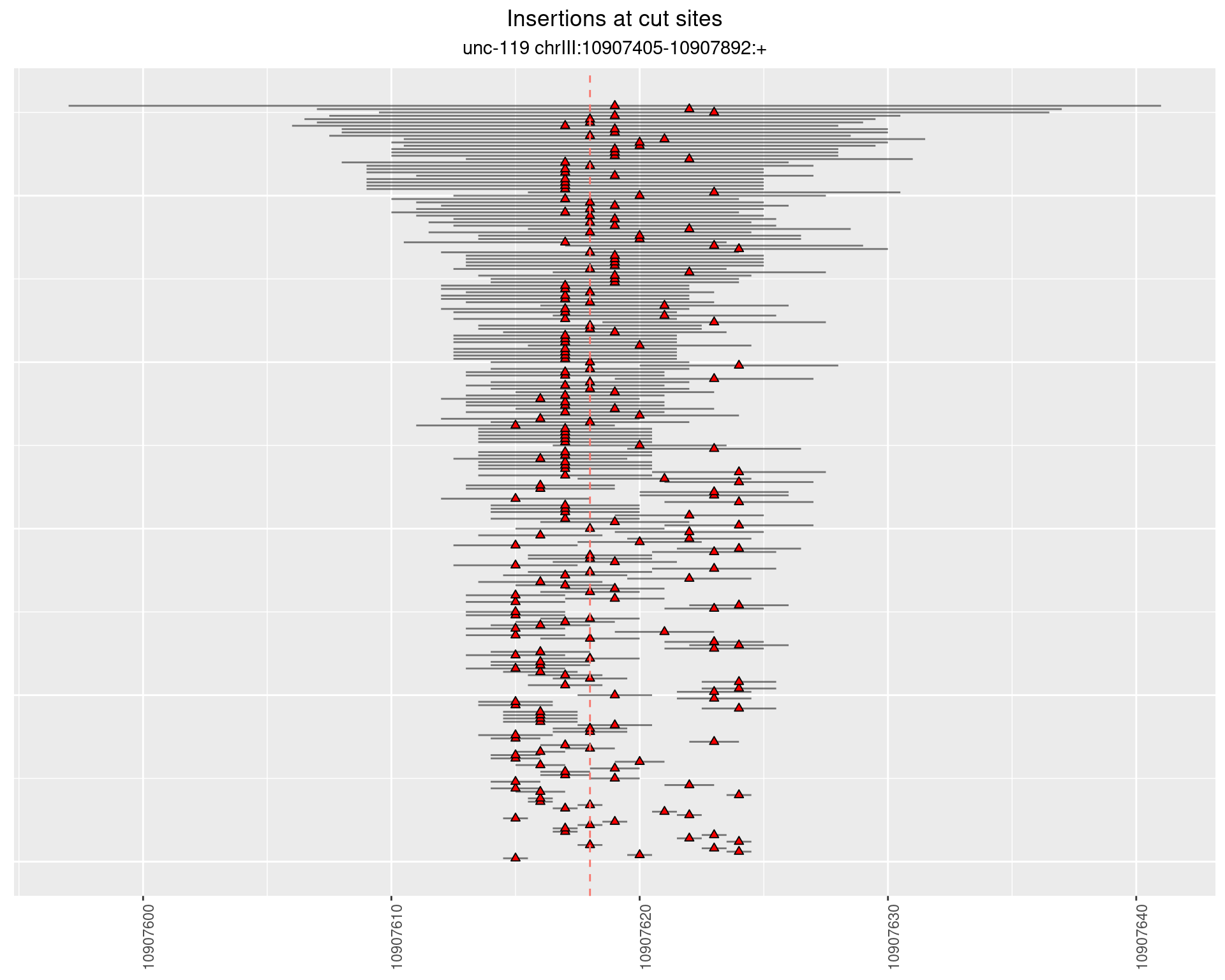
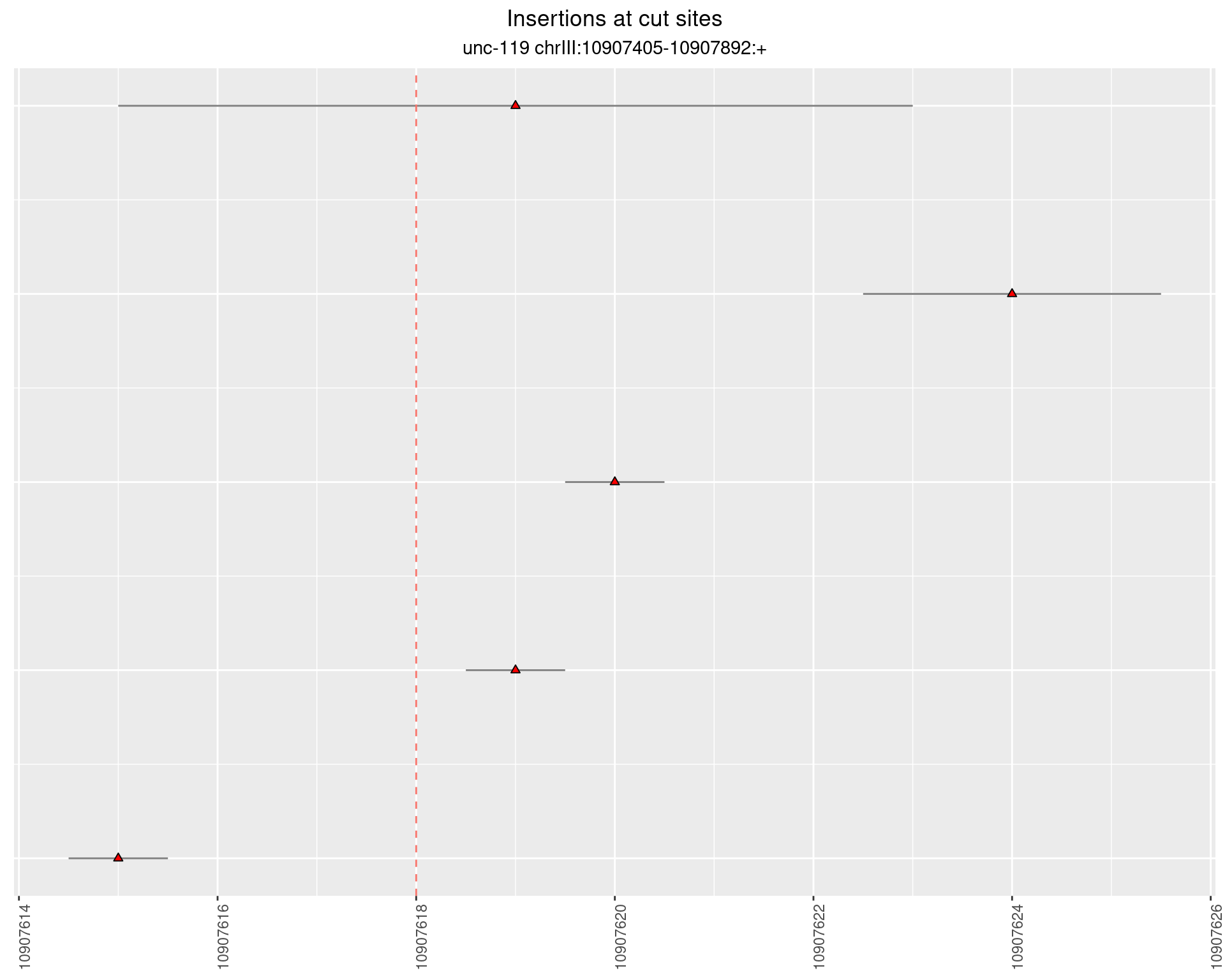
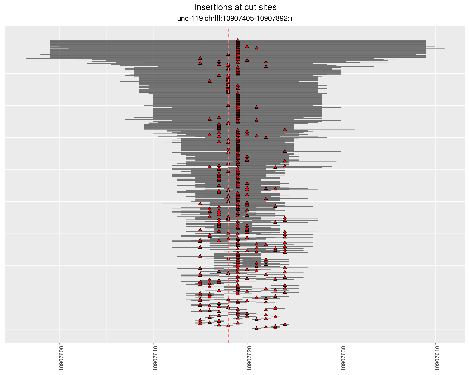
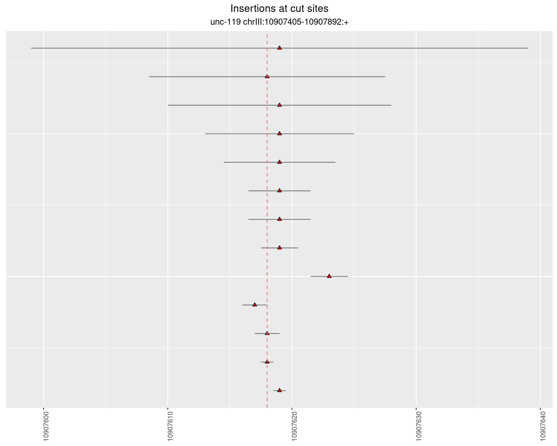
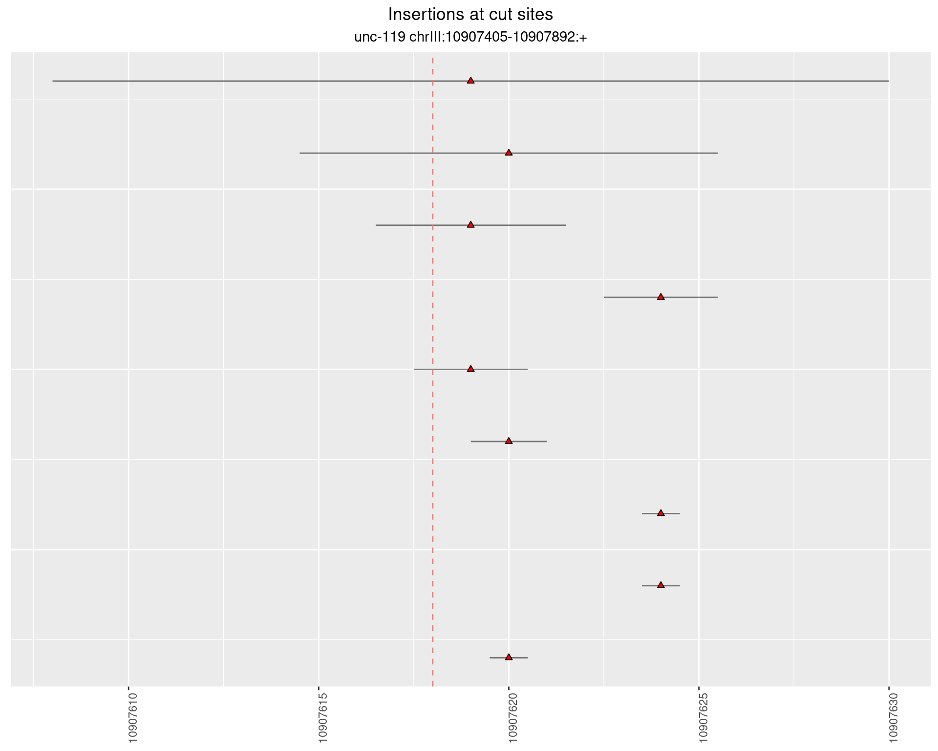
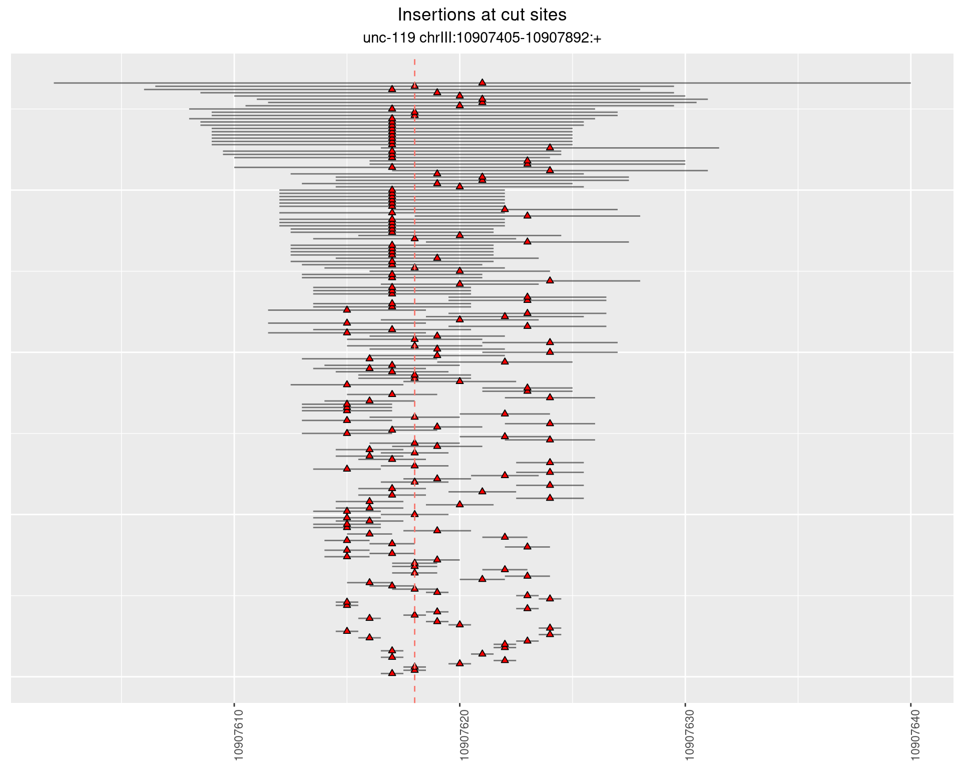
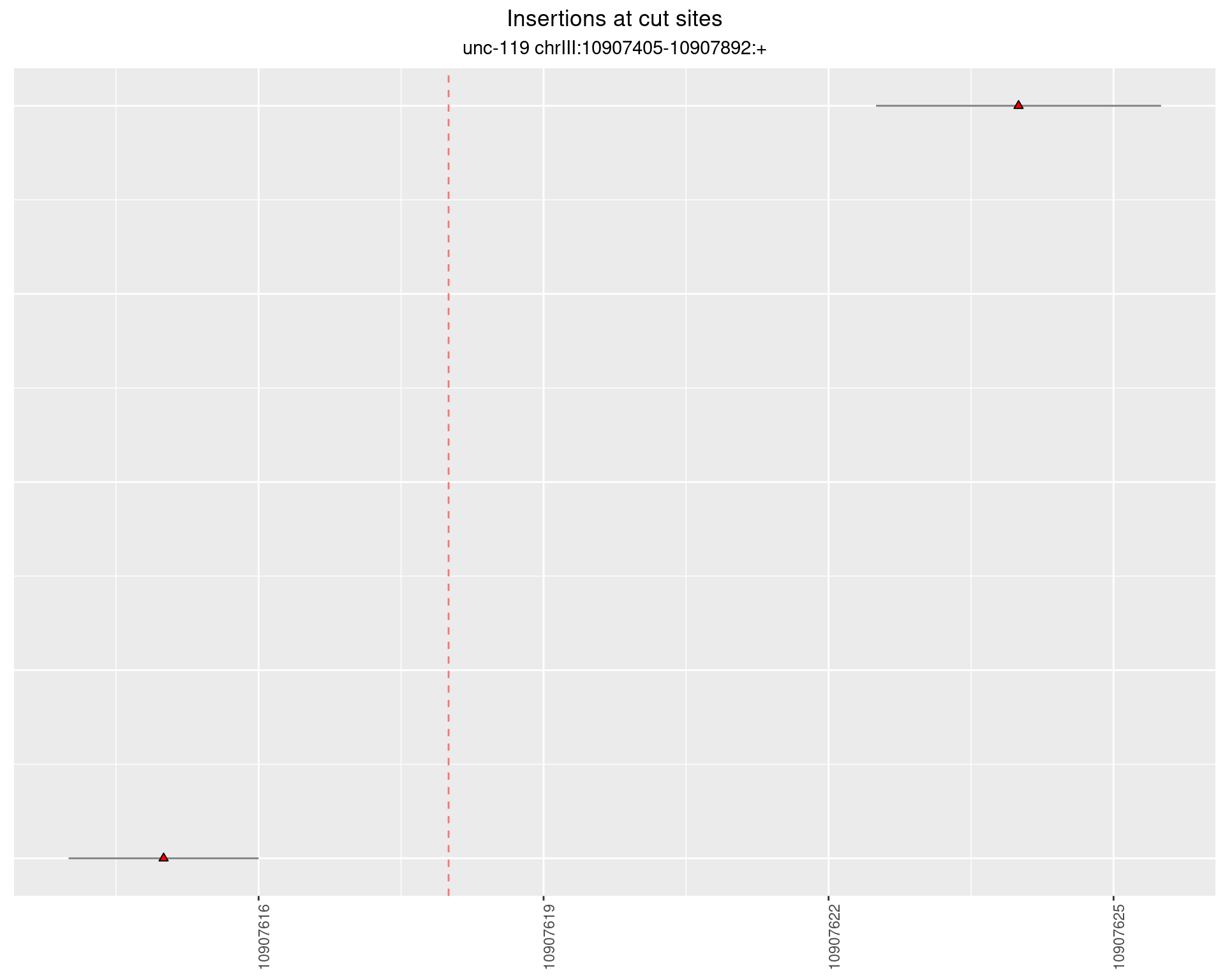
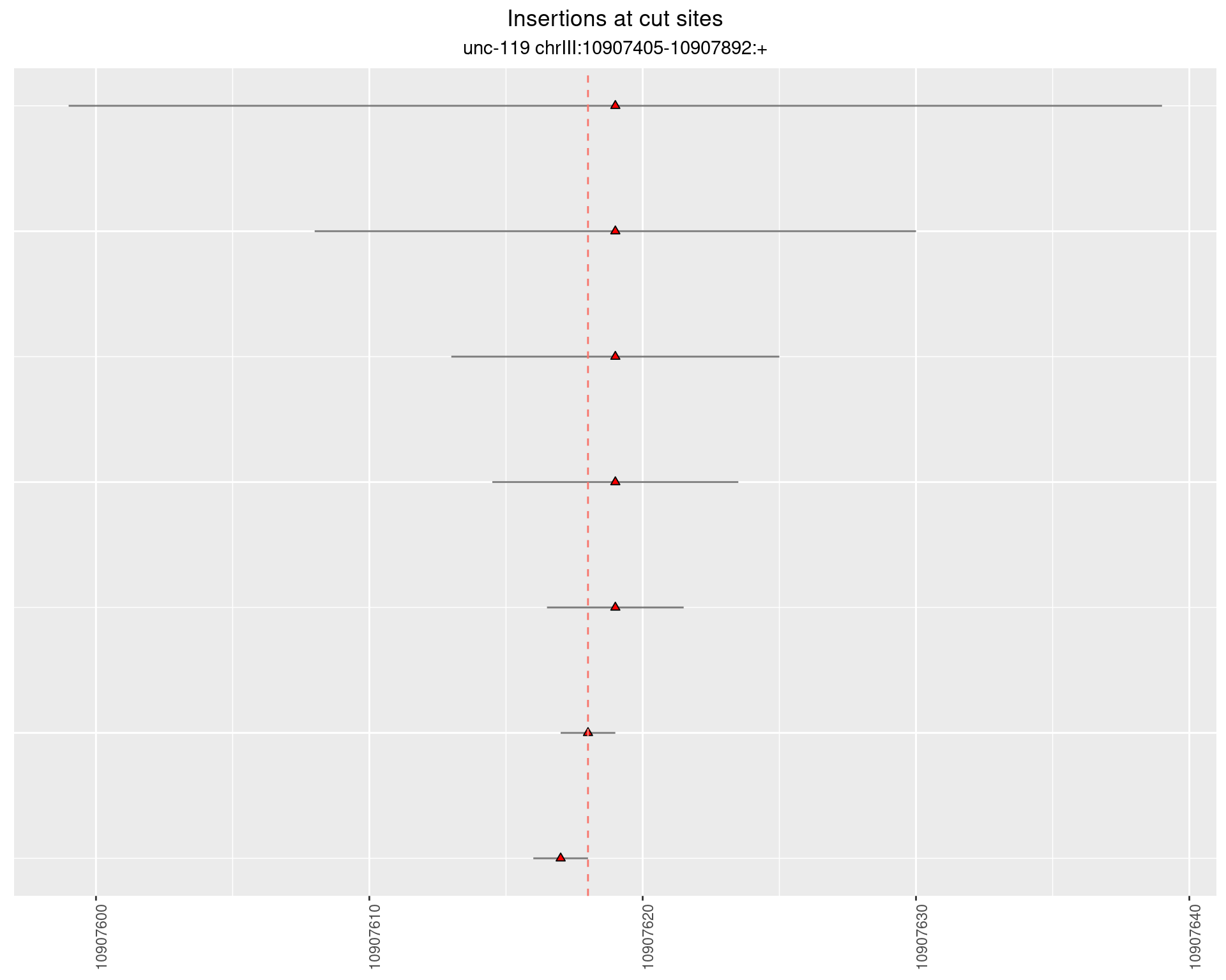
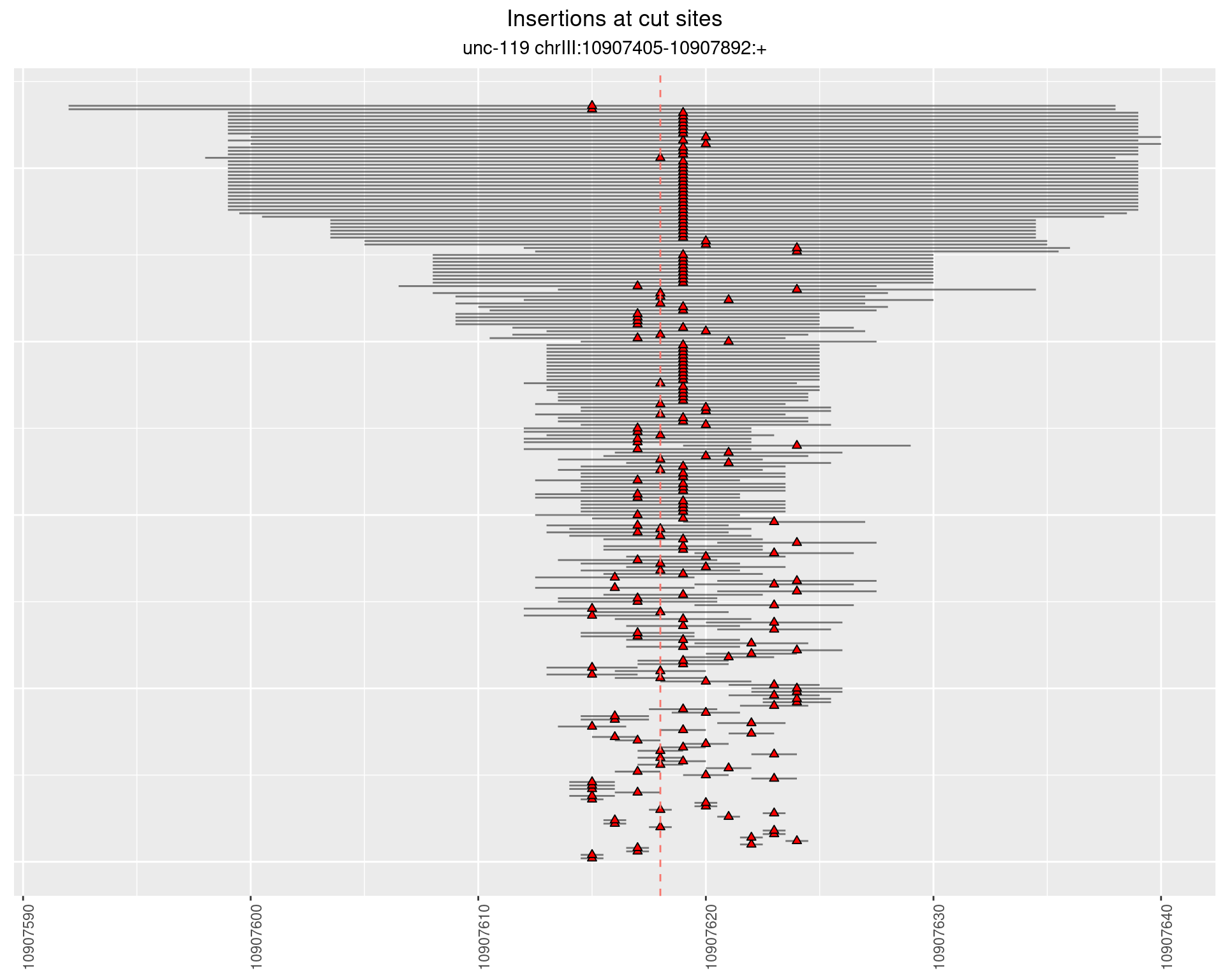
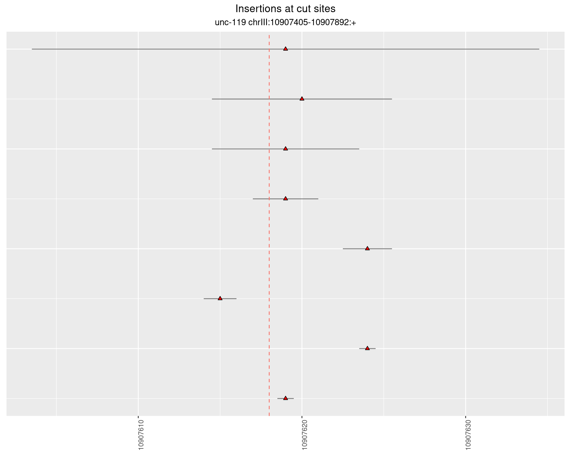
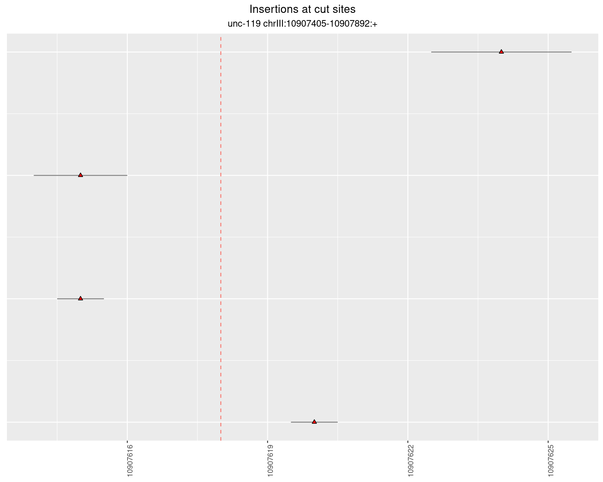
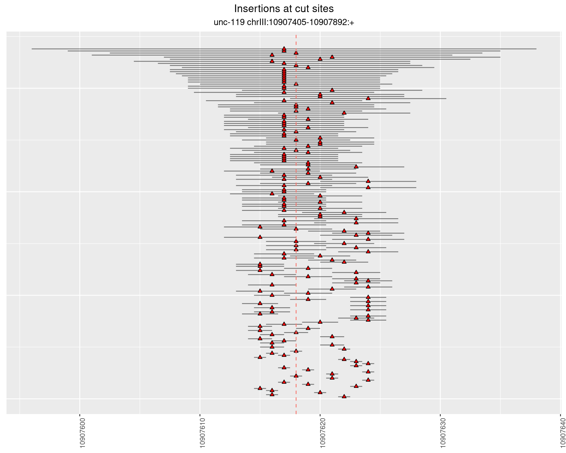
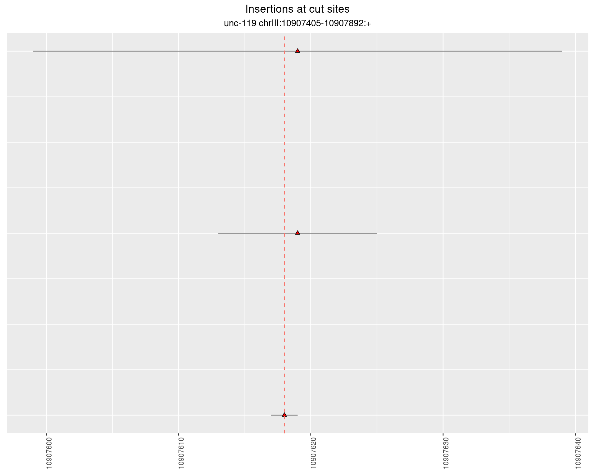
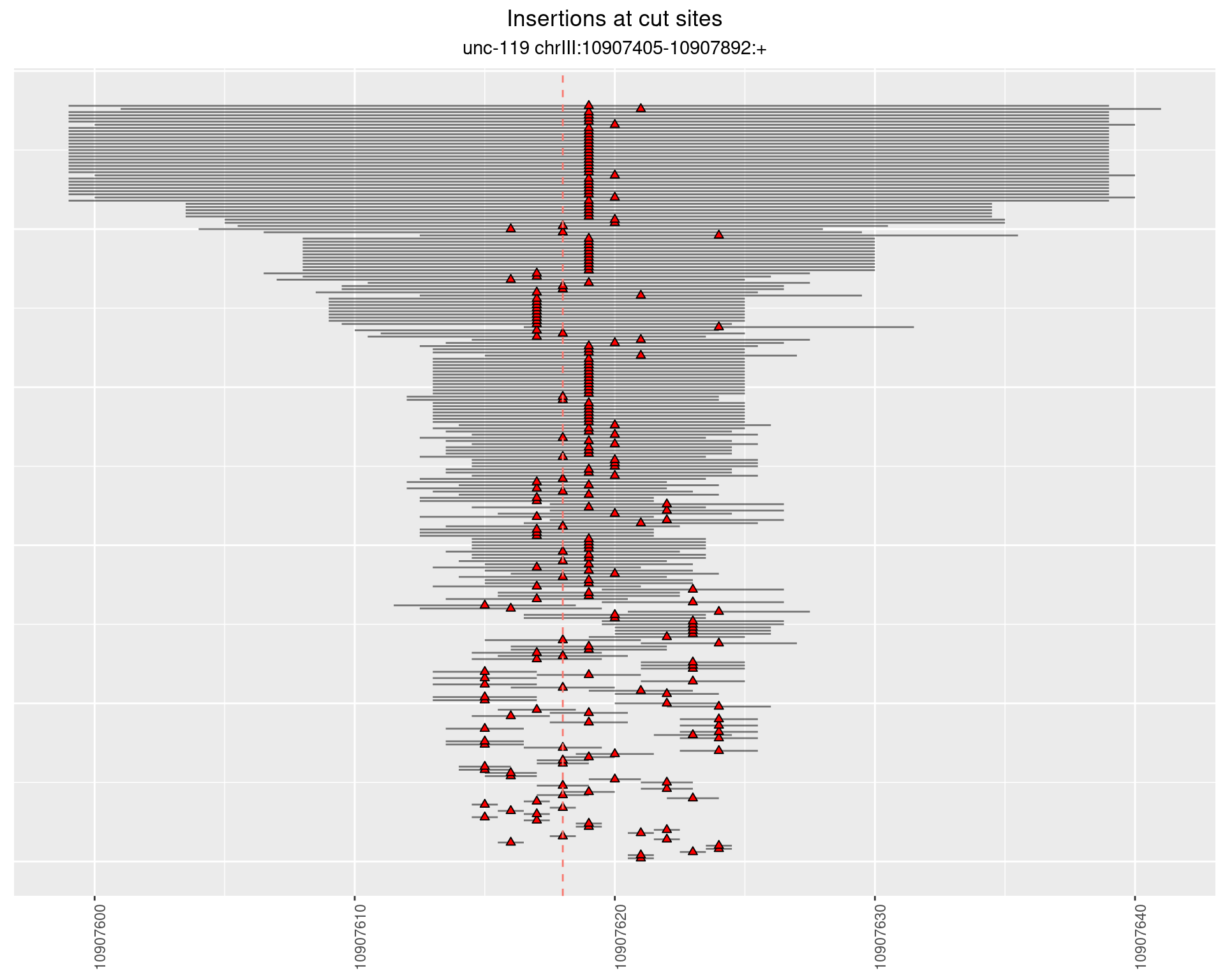
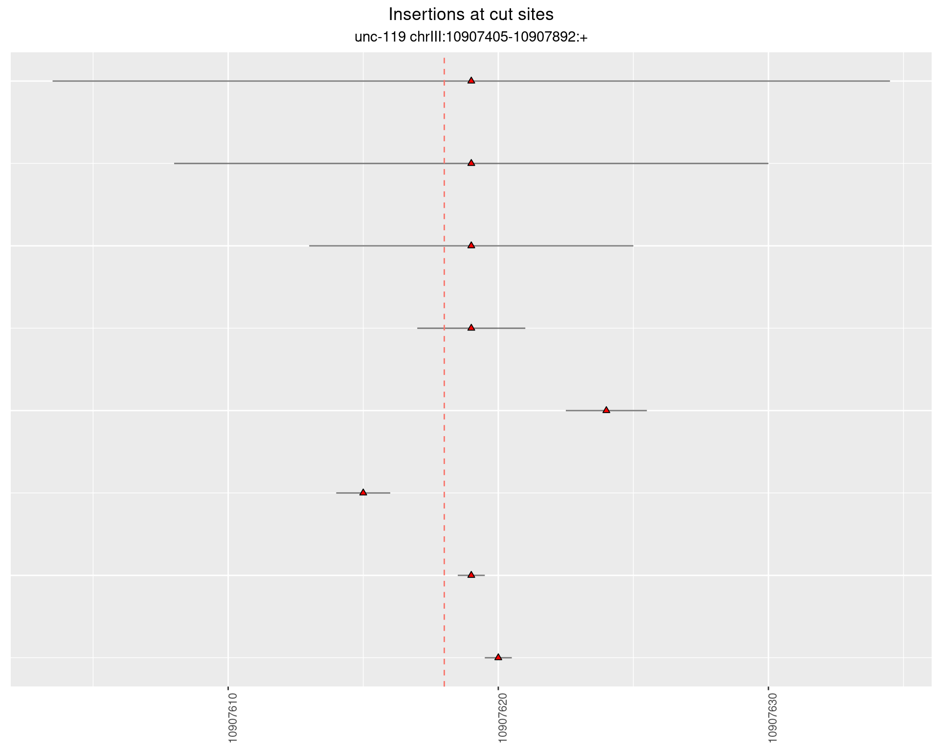
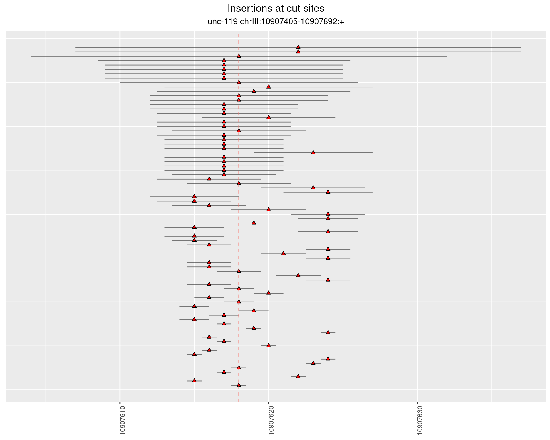
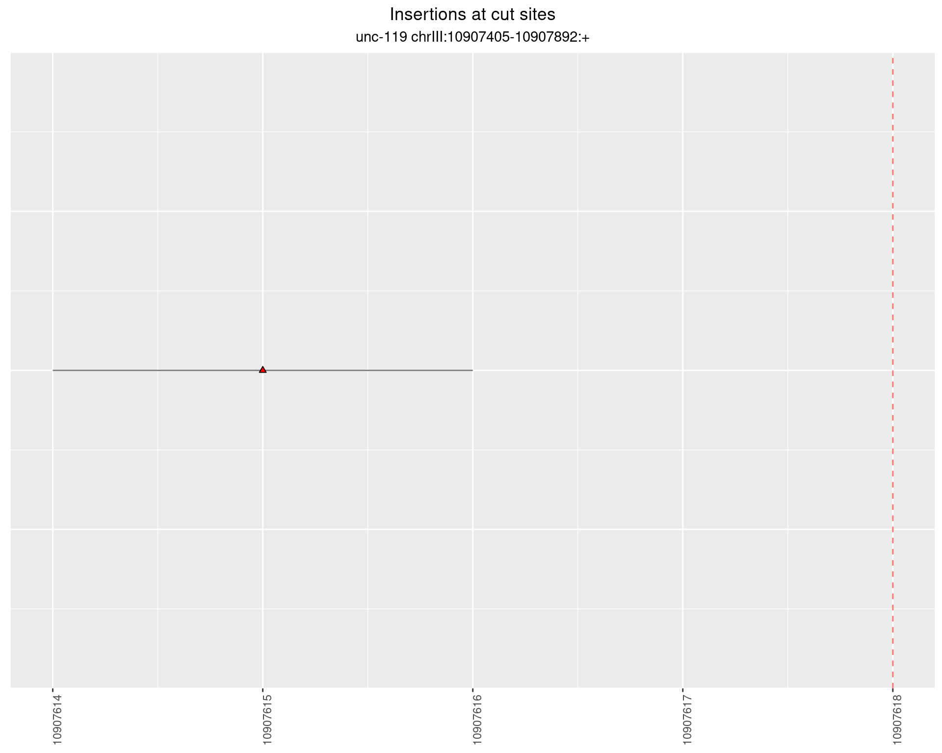
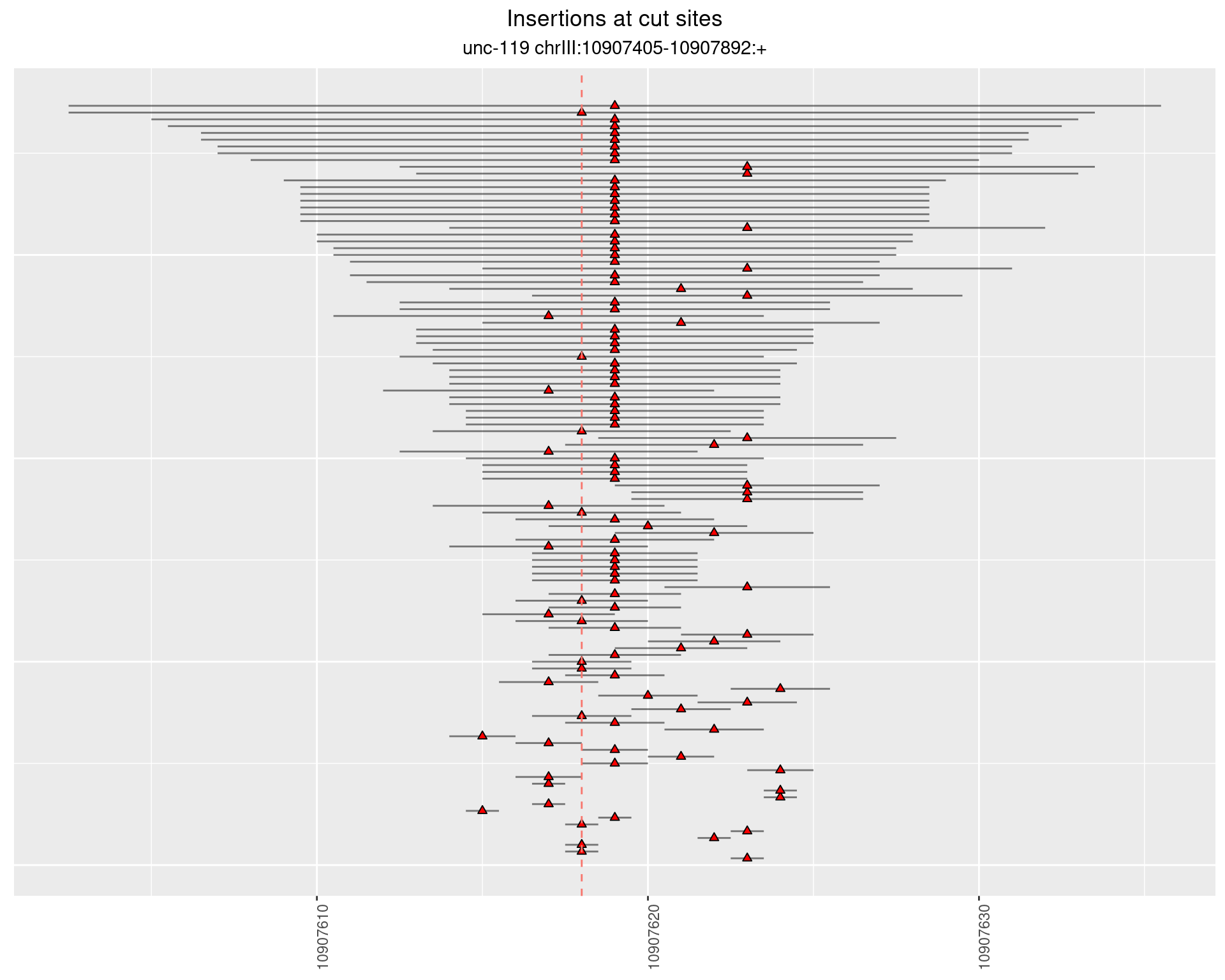
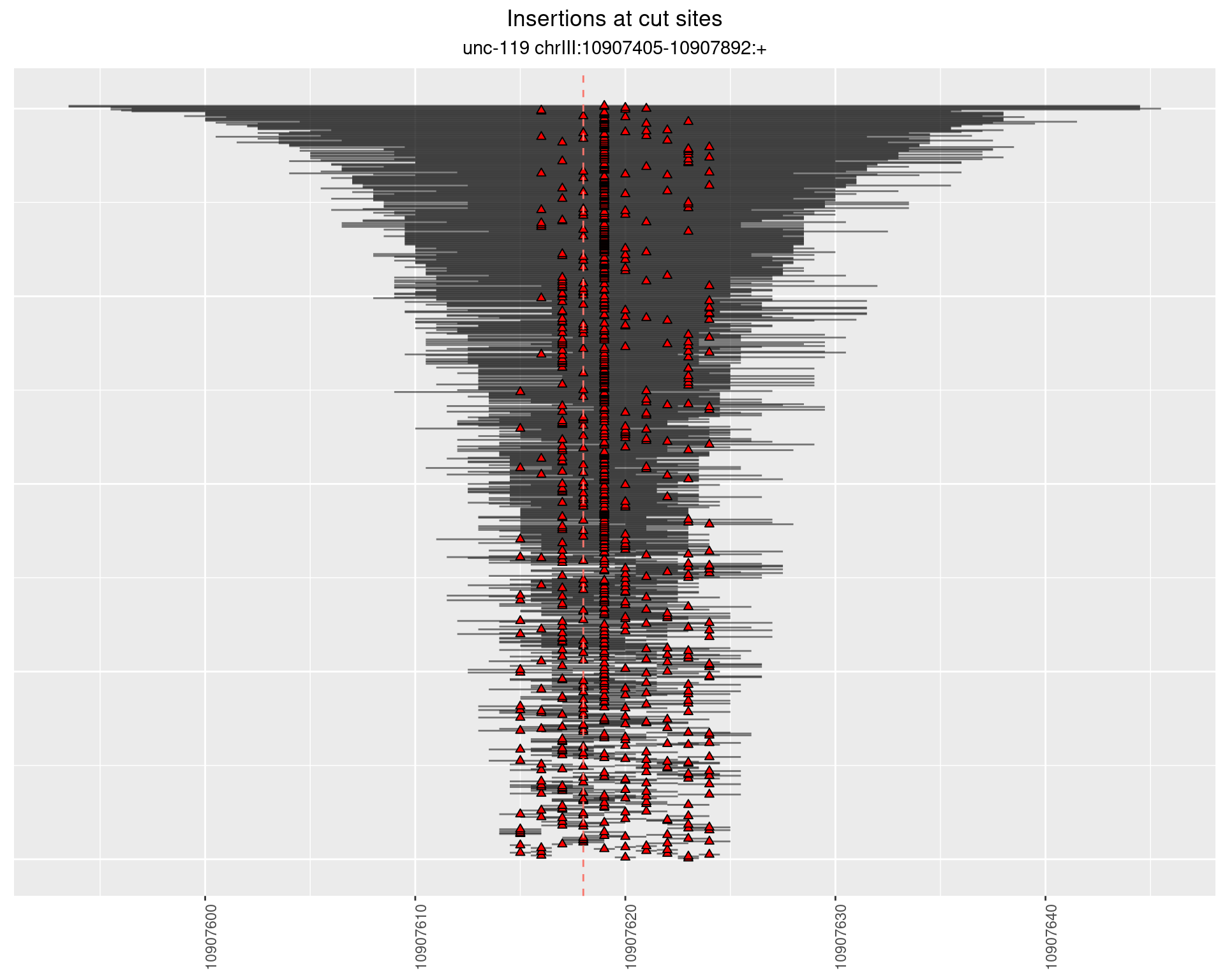
2 Insertion diversity at cut sites
These plots show the diversity of insertions at the cut sites taking into account the actual sequence that is inserted.
## import insertions data (that contains inserted sequences, too) and make some summary plots
insertions <- as.data.table(do.call(rbind, lapply(1:nrow(sampleSheet), function(i) {
  sampleName <- sampleSheet[i, 'sample_name']

  f <- file.path(pipeline_output_dir, 'indels', sampleName, paste0(sampleName, '.insertedSequences.tsv'))
  if(file.exists(f)) {
    dt <- data.table::fread(f)
    dt$sample <- sampleName
    dt$end <- dt$start
    return(dt)
  } else {
    warning("Can't open .insertedSequences.tsv file for sample ",sampleName,
            " at ",f,"\n")
    return(NULL)
  }
})))

#collapse insertions
insertions <- insertions[,length(name),
                         by = c('seqname', 'sample', 'start',
                                'end', 'insertedSequence',
                                'insertionWidth')]
colnames(insertions)[7] <- 'ReadSupport'

# get alignment coverage - will need for insertion coverage
alnCoverage <- importSampleBigWig(pipeline_output_dir,
                                  sampleSheet$sample_name, ".alnCoverage.bigwig")

insertions <- do.call(rbind, lapply(unique(insertions$sample), function(s) {
  do.call(rbind, lapply(unique(insertions[sample == s]$seqname), function(chr) {
    dt <- insertions[sample == s & seqname == chr]
    dt$coverage <- as.vector(alnCoverage[[s]][[chr]])[dt$start]
    return(dt)
  }))
}))

#compute frequency value for each insertion
#(number of reads supporting the insertion divided by coverage at insertion site)
insertions$freq <- insertions$ReadSupport/insertions$coverage

#find overlaps with cut sites
insertions <- cbind(insertions, overlapCutSites(indels = insertions, cutSites = cutSites))

# for each sample, find the guides used in the sample and find out if the indels overlap cut sites
# warnings: only restrict to the cut sites relevant for the sample
# warnings: if the sample is untreated, then we check overlaps for all cut sites
# for the corresponding amplicon
insertions <- do.call(rbind, lapply(unique(insertions$sample), function(sampleName) {
  dt <- insertions[sample == sampleName]
  sgRNAs <- sampleGuides[[sampleName]]
  dt$atCutSite <- apply(subset(dt, select = sgRNAs), 1, function(x) sum(x > 0) > 0)
  return(dt)
}))
plotInsertions <- function(dt, cutSites, sgRNAs) {
#first randomize the order (to avoid sorting by start position)
dt <- dt[sample(1:nrow(dt), nrow(dt))]
#sort insertions by width of insertion
dt <- dt[order(insertionWidth)]
dt$linePos <- 1:nrow(dt)
ggplot2::ggplot(dt, aes(x = linePos, ymin = start - insertionWidth/2,
ymax = start + insertionWidth/2)) +
geom_linerange(size = 0.5, alpha = 0.5) +
geom_point(aes(x = linePos, y = start), shape = 24, fill = 'red') +
geom_hline(data = as.data.frame(cutSites[cutSites$name %in% sgRNAs,]),
aes(yintercept = start, color = name), linetype = 'dashed', show.legend = FALSE) +
theme(axis.text.y = element_blank(),
axis.title.y = element_blank(),
axis.title.x = element_blank(),
axis.ticks.y = element_blank(),
axis.text.x = element_text(angle = 90),
plot.title = element_text(hjust = 0.5),
plot.subtitle = element_text(hjust = 0.5)) +
scale_y_continuous(sec.axis = dup_axis(breaks = cutSites[cutSites$sgRNA %in% sgRNAs,]$cutSite,
labels = cutSites[cutSites$sgRNA %in% sgRNAs,]$sgRNA)) +
coord_flip()
}
insertions$freqInterval <- cut_interval(log10(insertions$freq), length = 1)
plots <- lapply(unique(insertions$sample), function(sampleName) {
dt <- insertions[sample == sampleName & atCutSite == TRUE]
if(nrow(dt) == 0) {
return(NULL)
}
#dt$freqInterval <- cut_interval(log10(dt$freq), length = 1)
#segment plots with different frequency thresholds
segmentPlots <- lapply(unique(as.character(dt$freqInterval)), function(x) {
if(nrow(dt[freqInterval == x]) > 0) {
p <- plotInsertions(dt[freqInterval == x], cutSites, sampleGuides[[sampleName]])
p <- p + labs(title = 'Insertions at cut sites',
subtitle = paste(targetName, targetRegion))
} else {
p <- NULL
}
return(p)
})
names(segmentPlots) <- lapply(unique(as.character(dt$freqInterval)), function(x) {
paste(10^(as.numeric(unlist(strsplit(sub("(\\[|\\()(.+)(\\]|\\))", "\\2", x), ',')))),
collapse = ' - ')
})
return(segmentPlots)
})
names(plots) <- unique(insertions$sample)# folder to save pdf versions of the segment plots
dirPath <- paste(targetName, 'Indel_Diversity.insertion_segment_plots', sep = '.')
if(!dir.exists(dirPath)) {
dir.create(dirPath)
}
for (sample in names(plots)) {
cat('## ',sample,'{.tabset .tabset-fade .tabset-pills}\n\n')
for(i in names(plots[[sample]])) {
cat('### Freq:',i,'\n\n')
p <- plots[[sample]][[i]]
if(!is.null(p)) {
print(p)
ggsave(filename = file.path(dirPath, paste(sample, 'freq', i, 'pdf', sep = '.')),
plot = p, width = 10, height = 8, units = 'in')
} else {
cat("No plot to show\n\n")
}
cat("\n\n")
}
cat("\n\n")
}2.1 gen_24C_F2_unc-119_N2
2.1.1 Freq: 1e-06 - 1e-05
2.1.2 Freq: 1e-05 - 1e-04
2.2 gen_24C_F2_unc-119_sg1
2.2.1 Freq: 1e-04 - 0.001
2.2.2 Freq: 1e-05 - 1e-04
2.2.3 Freq: 1e-06 - 1e-05
2.3 gen_24C_F3_unc-119_N2
2.3.1 Freq: 1e-06 - 1e-05
2.3.2 Freq: 1e-05 - 1e-04
2.4 gen_24C_F3_unc-119_sg1
2.4.1 Freq: 1e-06 - 1e-05
2.4.2 Freq: 1e-04 - 0.001
2.4.3 Freq: 1e-05 - 1e-04
2.5 gen_24C_F4_unc-119_N2
2.5.1 Freq: 1e-06 - 1e-05
2.5.2 Freq: 1e-05 - 1e-04
2.6 gen_24C_F4_unc-119_sg1
2.6.1 Freq: 1e-04 - 0.001

2.6.2 Freq: 1e-05 - 1e-04
2.6.3 Freq: 1e-06 - 1e-05
2.7 gen_24C_F5_unc-119_N2
2.7.1 Freq: 1e-06 - 1e-05
2.7.2 Freq: 1e-05 - 1e-04
2.8 gen_24C_F5_unc-119_sg1
2.8.1 Freq: 1e-04 - 0.001
2.8.2 Freq: 1e-05 - 1e-04
2.8.3 Freq: 1e-07 - 1e-06
2.8.4 Freq: 1e-06 - 1e-05
2.9 gen_16C_F2_unc-119_N2
2.9.1 Freq: 1e-06 - 1e-05
2.9.2 Freq: 1e-05 - 1e-04
2.10 gen_16C_F2_unc-119_sg1
2.10.1 Freq: 1e-04 - 0.001
2.10.2 Freq: 1e-06 - 1e-05
2.10.3 Freq: 1e-05 - 1e-04
2.11 gen_16C_F3_unc-119_N2
2.11.1 Freq: 1e-06 - 1e-05
2.11.2 Freq: 1e-05 - 1e-04
2.12 gen_16C_F3_unc-119_sg1
2.12.1 Freq: 1e-06 - 1e-05
2.12.2 Freq: 1e-04 - 0.001
2.12.3 Freq: 1e-05 - 1e-04
2.13 gen_16C_F4_unc-119_N2
2.13.1 Freq: 1e-06 - 1e-05
2.13.2 Freq: 1e-05 - 1e-04
2.14 gen_16C_F4_unc-119_sg1
2.14.1 Freq: 1e-04 - 0.001
2.14.2 Freq: 1e-06 - 1e-05
2.14.3 Freq: 1e-05 - 1e-04
2.15 gen_16C_F5_unc-119_N2
2.15.1 Freq: 1e-05 - 1e-04
2.15.2 Freq: 1e-06 - 1e-05
2.16 gen_16C_F5_unc-119_sg1
2.16.1 Freq: 1e-04 - 0.001
2.16.2 Freq: 1e-06 - 1e-05
2.16.3 Freq: 1e-05 - 1e-04
2.17 gen_1624C_F1_unc-119_N2
2.17.1 Freq: 1e-06 - 1e-05
2.17.2 Freq: 1e-05 - 1e-04
2.18 gen_1624C_F1_unc-119_sg1
2.18.1 Freq: 1e-05 - 1e-04
2.18.2 Freq: 1e-06 - 1e-05
2.18.3 Freq: 1e-04 - 0.001