Pairwise Comparison of Samples
Read config.yml for the locations of sample sheet, pipeline output and cut sites coordinates.
Reading Config File:
knitr::opts_chunk$set(echo = TRUE, warning = FALSE, message = FALSE)
suppressMessages(suppressWarnings(library(knitr)))
suppressMessages(suppressWarnings(library(ggplot2)))
suppressMessages(suppressWarnings(library(ggrepel)))
suppressMessages(suppressWarnings(library(data.table)))
suppressMessages(suppressWarnings(library(rtracklayer)))
suppressMessages(suppressWarnings(library(plotly)))
suppressMessages(suppressWarnings(library(GenomicRanges)))
suppressMessages(suppressWarnings(library(parallel)))
suppressMessages(suppressWarnings(library(pbapply)))
suppressMessages(suppressWarnings(library(DT)))

targetName <- params$target_name
config <- yaml::read_yaml('./config.yml')
sampleSheet <- data.table::fread(config$sample_sheet)
pipeline_output_dir <- config$pipeline_output_dir
cut_sites <- rtracklayer::import.bed(config$cut_sites_file)
sampleComparisons <- data.table::fread(config$comparisons_file)
Declare some common functions
importSampleBigWig <- function(pipeline_output_dir, samples, suffix = '.alnCoverage.bigwig') {
  sapply(simplify = F, USE.NAMES = T,
                      X = unique(as.character(samples)),
                      FUN = function(s) {
  f <- file.path(pipeline_output_dir, 'indels', s, paste0(s, suffix))
  if(file.exists(f)) {
    rtracklayer::import.bw(f, as = 'RleList')
  } else {
    stop("Can't find bigwig file for sample: ",s," at: ",
         "\n",f,"\n")
  }})
}

subsetRleListByRange <- function(input.rle, input.gr) {
  as.vector(input.rle[[seqnames(input.gr)]])[start(input.gr):end(input.gr)]
}


getReadsWithIndels <- function(pipeline_output_dir, samples) {
  readsWithIndels <- lapply(samples, function(sample) {
  dt <- data.table::fread(file.path(pipeline_output_dir,
                                                 'indels',
                                                 sample,
                                                 paste0(sample, ".reads_with_indels.tsv")))
  })
  names(readsWithIndels) <- samples
  return(readsWithIndels)
}

getIndels <- function(pipeline_output_dir, samples) {
  indels <- sapply(simplify = FALSE, samples, function(s) {
  f <- file.path(pipeline_output_dir,
                 'indels',
                 s,
                 paste0(s, ".indels.tsv"))
  if(file.exists(f)) {
    dt <- data.table::fread(f)
    dt$sample <- s
    return(dt)
  } else {
    stop("Can't open indels.tsv file for sample",s,
            "at",f,"\n")
  }})
  return(indels)
}
Subset sample sheet for those that match the target region of interest
targetName <- params$target_name
sampleSheet <- sampleSheet[target_name == targetName]
targetRegion <- as(sampleSheet[target_name == targetName]$target_region[1], 'GRanges')
comp <- sampleComparisons[target_name == targetName]
if(nrow(comp) == 0) {
  cat("No comparisons to make for target region:",targetName,"\n")
  knitr::knit_exit()
}

outputFolder <- file.path(pipeline_output_dir, "comparisons", targetName)
dir.create(outputFolder, showWarnings = FALSE, recursive = TRUE)
# combine get per-base scores for all samples in the comparison list
samples <- unique(c(comp$case_samples, comp$control_samples))
#get reads with indels
readsWithIndels <- getReadsWithIndels(pipeline_output_dir,
samples)
#per-base number of reads with an insertion at the site
insertionCounts <- sapply(readsWithIndels, function(dt) {
gr <- GenomicRanges::makeGRangesFromDataFrame(dt[indelType == 'I'])
return(GenomicAlignments::coverage(gr))
})
#per-base number of reads with a deletion at the site
deletionCounts <- sapply(readsWithIndels, function(dt) {
gr <- GenomicRanges::makeGRangesFromDataFrame(dt[indelType == 'D'])
return(GenomicAlignments::coverage(gr))
})
#per-base number of reads with a deletion/insertion at the site
indelCounts <- sapply(readsWithIndels, function(dt) {
gr <- GenomicRanges::makeGRangesFromDataFrame(dt)
return(GenomicAlignments::coverage(gr))
})
# alignment coverage
alnCoverage <- importSampleBigWig(pipeline_output_dir,
samples, ".alnCoverage.bigwig")
coverageStats <- do.call(rbind, lapply(samples, function(s) {
target_region <- as(sampleSheet[target_name == targetName & sample_name == s]$target_region, 'GRanges')
#combine coverage, insertion, deletion scores
#subset rlelist by target region
dt <- data.table::data.table(
'cov' = subsetRleListByRange(alnCoverage[[s]], target_region),
'ins' = subsetRleListByRange(insertionCounts[[s]], target_region),
'del' = subsetRleListByRange(deletionCounts[[s]], target_region),
'indel' = subsetRleListByRange(indelCounts[[s]], target_region)
)
dt$bp <- start(target_region):end(target_region)
dt$seqname <- as.character(GenomeInfoDb::seqnames(target_region))
dt$sample <- s
dt[is.na(dt)] <- 0
return(dt)
}))comparePerBaseCounts <- function(coverageStats, caseSample, controlSample, indelType) {
case <- coverageStats[sample == caseSample,]
control <- coverageStats[sample == controlSample,]
#calculate fold-change per base
caseCov <- case[['cov']]
caseScore <- case[[indelType]]
controlCov <- control[['cov']]
controlScore <- control[[indelType]]
A <- ifelse(controlCov > 0, controlScore/controlCov, 0)
B <- ifelse(caseCov > 0, caseScore/caseCov, 0)
#percent difference between case and control
difference <- B - A
#p values - for each base, compare indel probabilities
#and get a fisher exact's p value
cl <- parallel::makeForkCluster(4)
results <- do.call(rbind, pbapply::pblapply(cl = cl, 1:length(caseScore), function(i) {
#contingency matrix
M <- matrix(c(caseScore[i], controlScore[i],
caseCov[i] - caseScore[i], controlCov[i] - controlScore[i]), nrow = 2)
t <- fisher.test(M)
oddsRatio <- as.numeric(t$estimate)
pVal <- t$p.value
return(data.frame('seqname' = case$seqname[i], 'bp' = case$bp[i], 'oddsRatio' = oddsRatio, 'pval' = pVal))
}))
parallel::stopCluster(cl)
results$padj <- p.adjust(results$pval)
results <- merge(data.frame('bp' = case$bp,
'case' = caseSample,
'control' = controlSample,
'caseScore' = caseScore,
'caseCov' = caseCov,
'controlScore' = controlScore,
'controlCov' = controlCov,
'indelType' = indelType,
'difference' = difference), results, by = 'bp')
return(results)
}
results <- as.data.frame(do.call(rbind, lapply(X = comp$comparison,
FUN = function(x) {
r <- do.call(rbind, lapply(c('ins', 'del', 'indel'), function(indelType) {
comparePerBaseCounts(coverageStats = coverageStats,
caseSample = comp[comparison == x,]$case_samples,
controlSample = comp[comparison == x,]$control_samples,
indelType = indelType)
}))
r$comparison <- x
return(r)
})), stringsAsFactors = FALSE)
pdf(file = file.path(outputFolder, paste0(targetName, ".comparisons.plots.pdf")))
plots <- lapply(unique(results$comparison), function(x){
plots <- lapply(unique(results$indelType), function(indelType) {
df <- results[results$comparison == x & results$indelType == indelType,]
#segment the profiles and calculate average p-values in each segment
segments <- as.data.frame(fastseg::fastseg(df$difference))
segments$mean.padj <- sapply(1:nrow(segments), function(i) {
mean(df[df$bp >= segments[i, 'start'] & df$bp <= segments[i, 'end'],]$padj)
})
#map p-values to stars for visualisation
segments$label <- gtools::stars.pval(segments$mean.padj)
segments$start <- min(df$bp) + segments$start - 1
segments$end <- min(df$bp) + segments$end - 1
p <- ggplot(df, aes(x = bp, y = difference)) +
geom_point(aes(color = padj < 0.05)) +
geom_segment(data = segments, aes(x = start, xend = end,
y = seg.mean, yend = seg.mean)) +
geom_text(data = segments, aes(x = (start+end)/2, y = seg.mean,
label = label)) +
ggtitle(paste0("Case sample: ",unique(as.character(df$case)),
"\nControl sample: ",unique(as.character(df$control))),
subtitle = paste0("Indel type: ", indelType)) +
theme_bw()
print(p)
## print the 'difference' value for each base position as a bigwig file
#outfile <- file.path(workdir, paste0(ampliconName, '.comparison.',
# x, '.', indelType, '.bedgraph'))
# TODO: print big
return(p)
})
names(plots) <- unique(results$indelType)
return(plots)
})
names(plots) <- unique(results$comparison)
#close pdf connection
dev.off()## png
## 2#save stats to file
statsOutFile <- file.path(outputFolder, paste0(targetName, '.comparison.stats.tsv'))
write.table(x = results, file = statsOutFile, quote = FALSE, sep = '\t', row.names = FALSE)1 Significantly Affected Base Positions/Segments
out = NULL
for (comparison in names(plots)) {
  out = c(out, knitr::knit_expand(text='## Comparison {{comparison}} {.tabset} \n\n'))
  for (indelType in names(plots[[comparison]])) {
    p <- ggplotly(plots[[comparison]][[indelType]])
    out = c(out, knitr::knit_expand(text='### {{indelType}} \n\n {{p}} \n\n'))
  }
}
1.1 Comparison gen_plates_let-2_UTR_pool___F2_vs_N2 {.tabset}
1.1.1 ins
1.1.2 del
1.1.3 indel
1.2 Comparison gen_plates_let-2_UTR_pool_24C_plate3_vs_gen_plates_let-2_UTR_pool_F2 {.tabset}
1.2.1 ins
1.2.2 del
1.2.3 indel
1.3 Comparison gen_plates_let-2_UTR_pool_24C_plate5_vs_gen_plates_let-2_UTR_pool_F2 {.tabset}
1.3.1 ins
1.3.2 del
1.3.3 indel
1.4 Comparison gen_plates_let-2_UTR_pool_16C_plate3_vs_gen_plates_let-2_UTR_pool_F2 {.tabset}
1.4.1 ins
1.4.2 del
1.4.3 indel
1.5 Comparison gen_plates_let-2_UTR_pool_16C_plate5_vs_gen_plates_let-2_UTR_pool_F2 {.tabset}
1.5.1 ins
1.5.2 del
1.5.3 indel
1.6 Comparison gen_plates_let-2_UTR_pool_24C_plate5_vs_gen_plates_let-2_UTR_pool_16C_plate5 {.tabset}
1.6.1 ins
1.6.2 del
1.6.3 indel
1.7 Comparison gen_plates_let-2_UTR_pool_24C_plate3_vs_gen_plates_let-2_UTR_pool_16C_plate3 {.tabset}
1.7.1 ins
1.7.2 del
1.7.3 indel
2 Comparison of indel frequencies
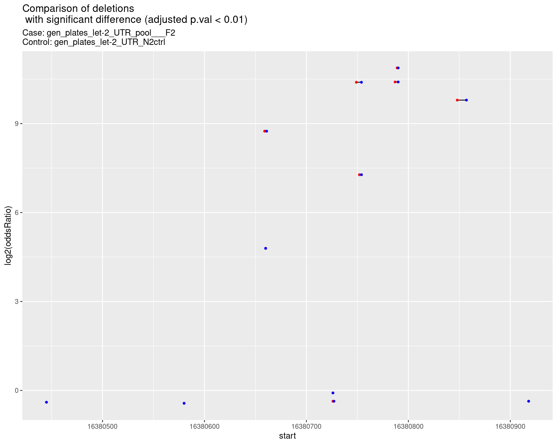
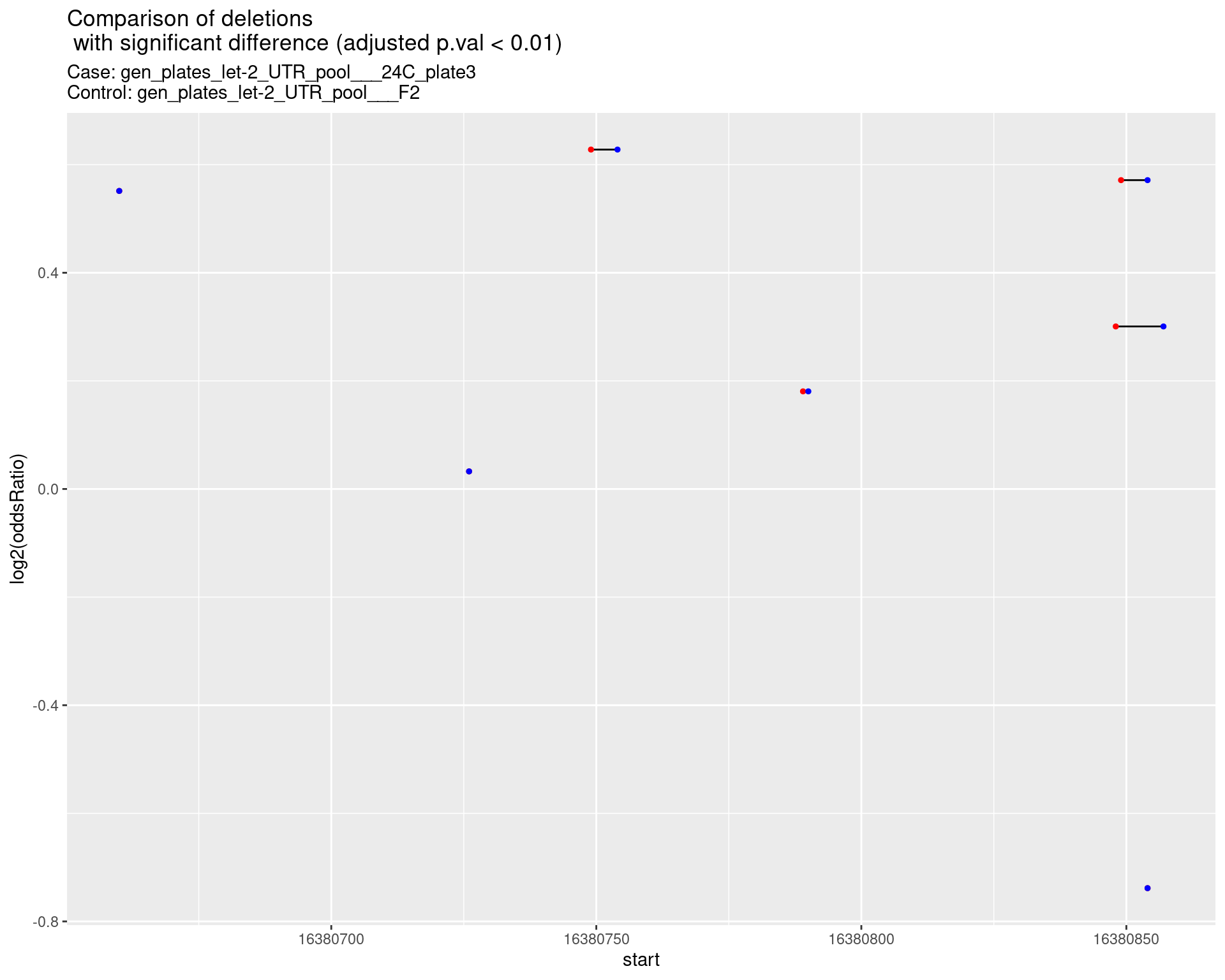
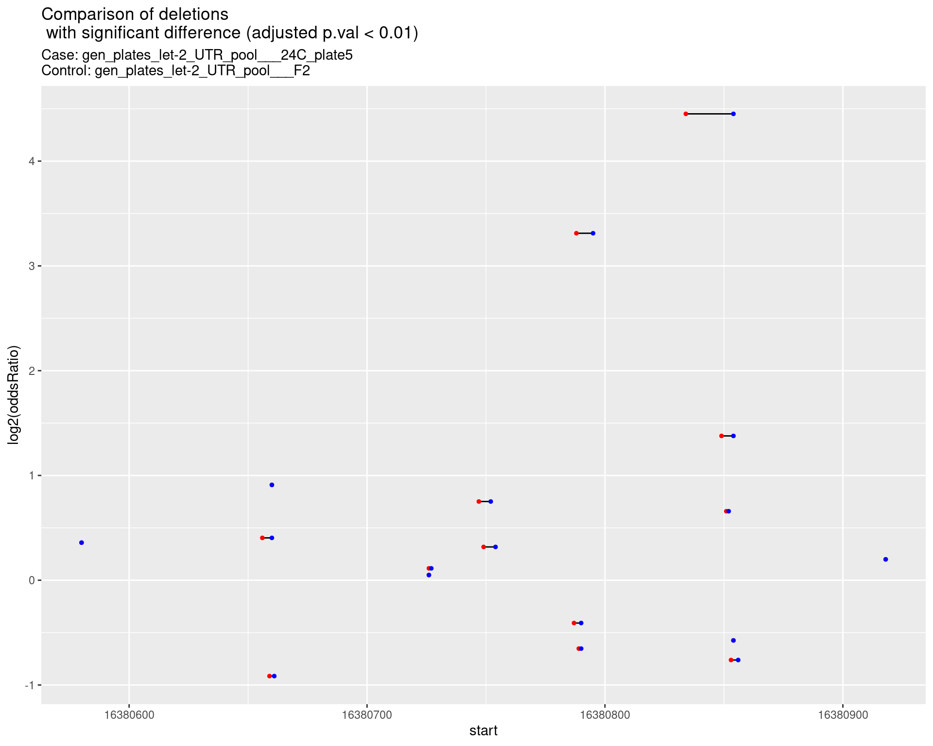
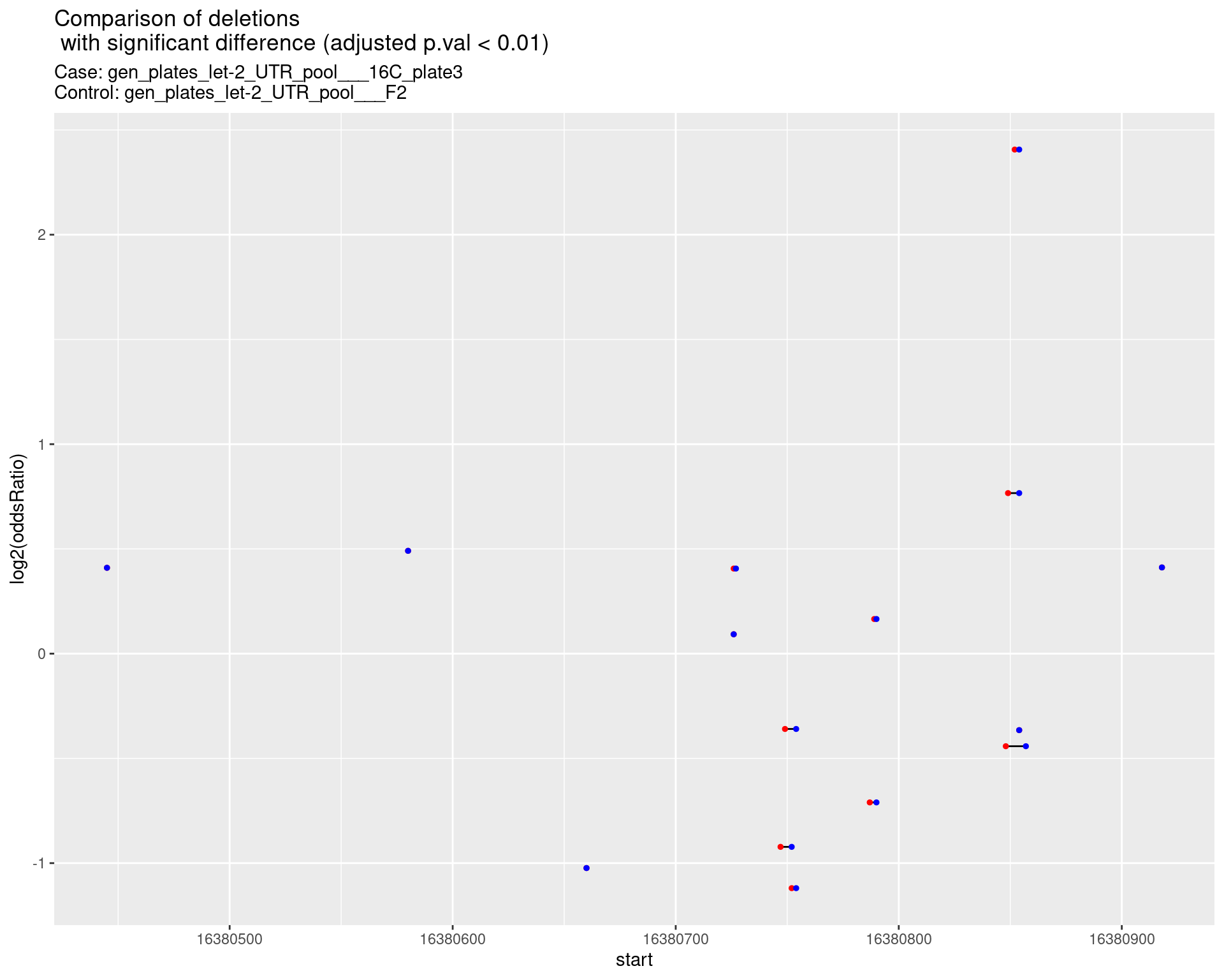
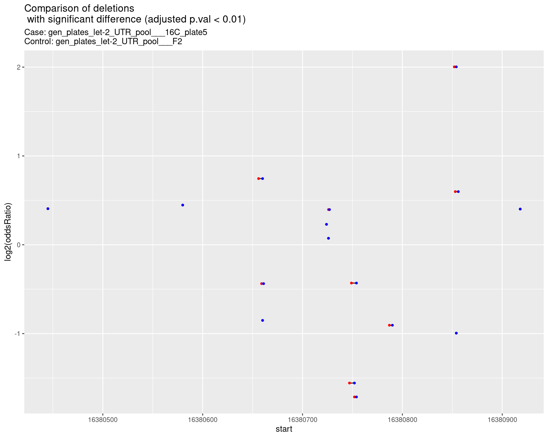
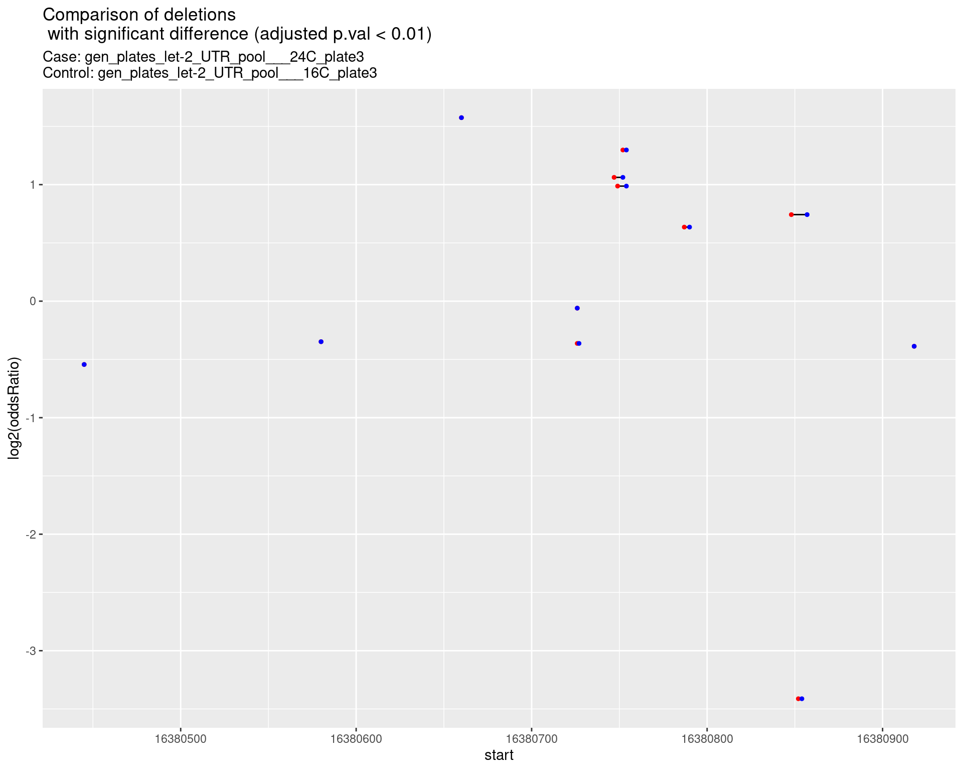
2.1 Deletion frequencies
First, get deletions and the coverage values for each deletion
samples <- unique(c(comp$case_samples, comp$control_samples))

deletions <- do.call(rbind, lapply(getIndels(pipeline_output_dir, samples),
                    function(dt) {
                      dt[indelType == 'D']
                    }))

#get deletions within the target region
deletions <- as.data.table(subsetByOverlaps(GRanges(deletions), targetRegion, ignore.strand = TRUE))

#create a table where each deletion found in all samples is represented for each sample
#whether or not the deletion is found in the corresponding sample

deletions <- data.table::melt(dcast.data.table(deletions, name ~ sample, value.var = 'ReadSupport'), id.vars = 'name')
#assign NA values to 0
deletions[is.na(value)]$value <- 0
colnames(deletions) <- c('name', 'sample', 'ReadSupport')

deletions <- cbind(do.call(rbind, strsplit(deletions$name, ':')), deletions)
colnames(deletions)[1:3] <- c('seqname', 'start', 'end')
deletions$start <- as.numeric(deletions$start)
deletions$end <- as.numeric(deletions$end)

#get max coverage at the bases spanned by each deletion
deletions <- do.call(rbind, lapply(unique(deletions$sample), function(s) {
  dt <- deletions[sample == s]

  #make sure the coverage values start from the first base position
  #if not, fill those positions up to first coverage value with zeroes
  coverage <- coverageStats[sample == s][order(bp)]
  coverage <- c(rep(0, coverage[1,]$bp - 1),
                coverage$cov)

  dt$coverage <- apply(dt, 1, function(x) {
    max(coverage[x[['start']]:x[['end']]])
  })
  return(dt)
}))
deletions$freq <- deletions$ReadSupport/deletions$coverage
Make plots to compare case versus control samples
#dt: deletions/insertions table
#minReadSupport mininum number of reads in sum of the samples
#minFreq minimum frequency in sum of the samples
# TODO: add minCoveragePercentile = 10
getSignificantIndels <- function(dt, caseSample, controlSample, minReadSupport = 5, minFreq = 10^-4) {
  #subset for control samples
  dt <- droplevels(dt[sample %in% c(caseSample, controlSample)])

  #independent filtering for read support
  dt <- dt[name %in% dt[,sum(ReadSupport), by = name][V1 > minReadSupport]$name]

  #independent filtering for frequency
  dt <- dt[name %in% dt[,sum(freq), by = name][V1 > minFreq]$name]

  if(nrow(dt) == 0) {
    cat("warning: getSignificantIndels => No significant indels left after filtering")
    return(NULL)
  }

  # median coverage values as integer
  dt$coverage <- as.integer(dt$coverage)

  case <- dt[sample == caseSample]
  ctrl <- dt[sample == controlSample]

  mdt <- merge(case[,c('name', 'ReadSupport', 'coverage')],
        ctrl[,c('name', 'ReadSupport', 'coverage')],
        by = 'name', all = TRUE)

  #convert NA values to 0
  mdt[is.na(mdt)] <- 0

  results <- cbind(mdt, do.call(rbind, apply(mdt, 1, function(x) {
    #add a constant value (5) to each category to avoid Inf values
    x <- as.numeric(x[2:5])
    test <- fisher.test(matrix(c(x[1], x[3],
                                 x[2] - x[1], x[4] - x[3]), nrow = 2) + 1,
                        alternative = 'two.sided')
    return(data.frame('pval' = test$p.value, 'oddsRatio' = as.numeric(test$estimate)))
  })))

  results$padj <- p.adjust(results$pval, method = 'BH')

  return(results)
}

plots <- pbapply::pblapply(unique(comp$comparison), function(cmp) {
  caseSample <- comp[comparison == cmp]$case_samples
  controlSample <- comp[comparison == cmp]$control_samples

  #get significance values for each deletion
  sig <- getSignificantIndels(dt = as.data.table(subsetByOverlaps(as(deletions, "GRanges"), targetRegion)),
                              caseSample = caseSample,
                              controlSample = controlSample,
                              minReadSupport = 5,
                              minFreq = 10^-3)
  if(is.null(sig)) {
    return(list("volcano_plot" = NULL, "segment_plot" = NULL))
  }
  results <- merge(unique(deletions[,c('seqname','start', 'end', 'name')]),
                   sig,
                   by = 'name')
  #save results table
  write.table(x = results[order(pval)],
              file = file.path(outputFolder, paste0(targetName, ".comparison.",
                                               cmp, ".stats.deletions.tsv")),
              row.names = FALSE, quote = FALSE, sep = '\t')

  #make a segment plot of deletions
  p <- ggplot(results[padj < 0.01]) +
    geom_linerange(aes(x = log2(oddsRatio), ymin = start, ymax = end)) +
    geom_point(data = results[padj < 0.01], aes(x = log2(oddsRatio), y = start), size = 1, color = 'red') +
    geom_point(data = results[padj < 0.01], aes(x = log2(oddsRatio), y = end), size = 1, color = 'blue') +
    ggtitle(label = "Comparison of deletions\n with significant difference (adjusted p.val < 0.01)",
            subtitle = paste0("Case: ",caseSample, "\nControl: ",controlSample)) +
    coord_flip()

  return(list("segment_plot" = p))
})
names(plots) <- unique(comp$comparison)
for (cmp in names(plots)) {
cat('### Comparison:',cmp,'{.tabset}\n\n')
for(i in names(plots[[cmp]])) {
cat('#### ',i,'\n\n')
p <- plots[[cmp]][[i]]
if(!is.null(p)) {
print(p)
} else {
cat("No plot to show\n\n")
}
cat("\n\n")
}
cat("\n\n")
}2.1.1 Comparison: gen_plates_let-2_UTR_pool___F2_vs_N2 {.tabset}
2.1.1.1 segment_plot
2.1.2 Comparison: gen_plates_let-2_UTR_pool_24C_plate3_vs_gen_plates_let-2_UTR_pool_F2 {.tabset}
2.1.2.1 segment_plot
2.1.3 Comparison: gen_plates_let-2_UTR_pool_24C_plate5_vs_gen_plates_let-2_UTR_pool_F2 {.tabset}
2.1.3.1 segment_plot
2.1.4 Comparison: gen_plates_let-2_UTR_pool_16C_plate3_vs_gen_plates_let-2_UTR_pool_F2 {.tabset}
2.1.4.1 segment_plot
2.1.5 Comparison: gen_plates_let-2_UTR_pool_16C_plate5_vs_gen_plates_let-2_UTR_pool_F2 {.tabset}
2.1.5.1 segment_plot
2.1.6 Comparison: gen_plates_let-2_UTR_pool_24C_plate5_vs_gen_plates_let-2_UTR_pool_16C_plate5 {.tabset}
2.1.6.1 segment_plot

2.1.7 Comparison: gen_plates_let-2_UTR_pool_24C_plate3_vs_gen_plates_let-2_UTR_pool_16C_plate3 {.tabset}
2.1.7.1 segment_plot
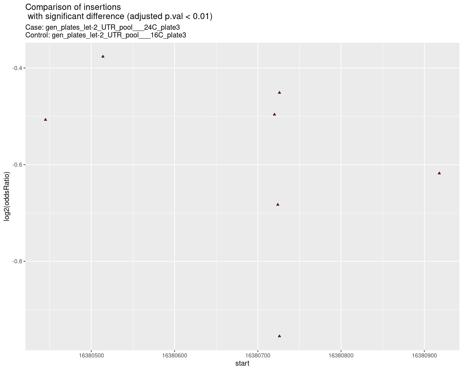
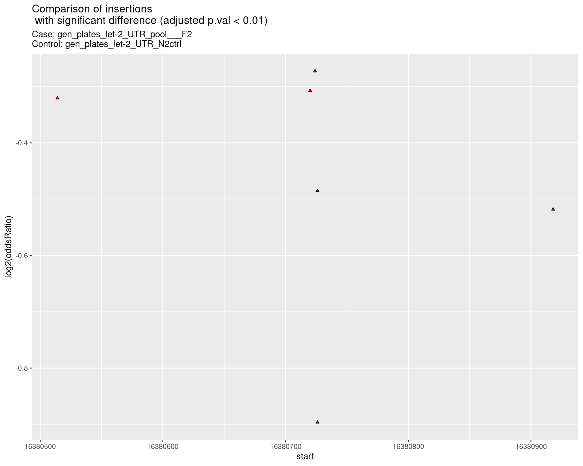
2.2 Insertion frequencies
## import insertions data (that contains inserted sequences, too) and make some summary plots
insertions <- as.data.table(do.call(rbind, lapply(1:nrow(sampleSheet), function(i) {
  sampleName <- sampleSheet[i, 'sample_name']

  f <- file.path(pipeline_output_dir, 'indels', sampleName, paste0(sampleName, '.insertedSequences.tsv'))
  if(file.exists(f)) {
    dt <- data.table::fread(f)
    dt$sample <- sampleName
    dt$end <- dt$start
    return(dt)
  } else {
    warning("Can't open .insertedSequences.tsv file for sample ",sampleName,
            " at ",f,"\n")
    return(NULL)
  }
})))

#collapse insertions
insertions <- insertions[,length(name),
                         by = c('seqname', 'sample', 'start',
                                'end', 'insertedSequence',
                                'insertionWidth')]
colnames(insertions)[7] <- 'ReadSupport'

# get alignment coverage - will need for insertion coverage
alnCoverage <- importSampleBigWig(pipeline_output_dir,
                                  sampleSheet$sample_name, ".alnCoverage.bigwig")

insertions <- do.call(rbind, lapply(unique(insertions$sample), function(s) {
  do.call(rbind, lapply(unique(insertions[sample == s]$seqname), function(chr) {
    dt <- insertions[sample == s & seqname == chr]
    dt$coverage <- as.vector(alnCoverage[[s]][[chr]])[dt$start]
    return(dt)
  }))
}))

#compute frequency value for each insertion
#(number of reads supporting the insertion divided by coverage at insertion site)
insertions$freq <- insertions$ReadSupport/insertions$coverage
insertions$name <- paste(insertions$seqname, insertions$start, insertions$insertedSequence, sep = ":")
Make plots to compare case versus control samples
plots <- pbapply::pblapply(unique(comp$comparison), function(cmp) {
  caseSample <- comp[comparison == cmp]$case_samples
  controlSample <- comp[comparison == cmp]$control_samples


  #get significance values for each insertion at the target region
  sig <- getSignificantIndels(dt = as.data.table(subsetByOverlaps(as(insertions, "GRanges"), targetRegion)),
                              caseSample = caseSample,
                              controlSample = controlSample,
                              minReadSupport = 5,
                              minFreq = 10^-3)
  if(is.null(sig)) {
    return(list("segment_plot" = NULL))
  }

  results <- merge(unique(insertions[,c('seqname','start', 'name')]),
                   sig,
                   by = 'name')

  #save results table
  write.table(x = results[order(pval)],
              file = file.path(outputFolder, paste0(targetName, ".comparison.",
                                               cmp, ".stats.insertions.tsv")),
              row.names = FALSE, quote = FALSE, sep = '\t')

  #make a segment plot of deletions
  results$insertionWidth <- sapply(strsplit(results$name, ":"), function(x) nchar(x[3]))
  p <- ggplot(results[padj < 0.01]) +
    geom_linerange(aes(x = log2(oddsRatio),
                       ymin = start - insertionWidth/2,
                       ymax = start + insertionWidth/2),
                   alpha = 0.5) +
    geom_point(data = results[padj < 0.01],
               aes(x = log2(oddsRatio), y = start),
               size = 1, shape = 24, fill = 'red') +
    ggtitle(label = "Comparison of insertions\n with significant difference (adjusted p.val < 0.01)",
            subtitle = paste0("Case: ",caseSample, "\nControl: ",controlSample)) +
    coord_flip()

  return(list("segment_plot" = p))
})
names(plots) <- unique(comp$comparison)
for (cmp in names(plots)) {
cat('### Comparison:',cmp,'{.tabset .tabset-pills .tabset-fade}\n\n')
for(i in names(plots[[cmp]])) {
cat('#### ',i,'\n\n')
p <- plots[[cmp]][[i]]
if(!is.null(p)) {
print(p)
} else {
cat("No plot to show\n\n")
}
cat("\n\n")
}
cat("\n\n")
}2.2.1 Comparison: gen_plates_let-2_UTR_pool___F2_vs_N2 {.tabset .tabset-pills .tabset-fade}
2.2.1.1 segment_plot
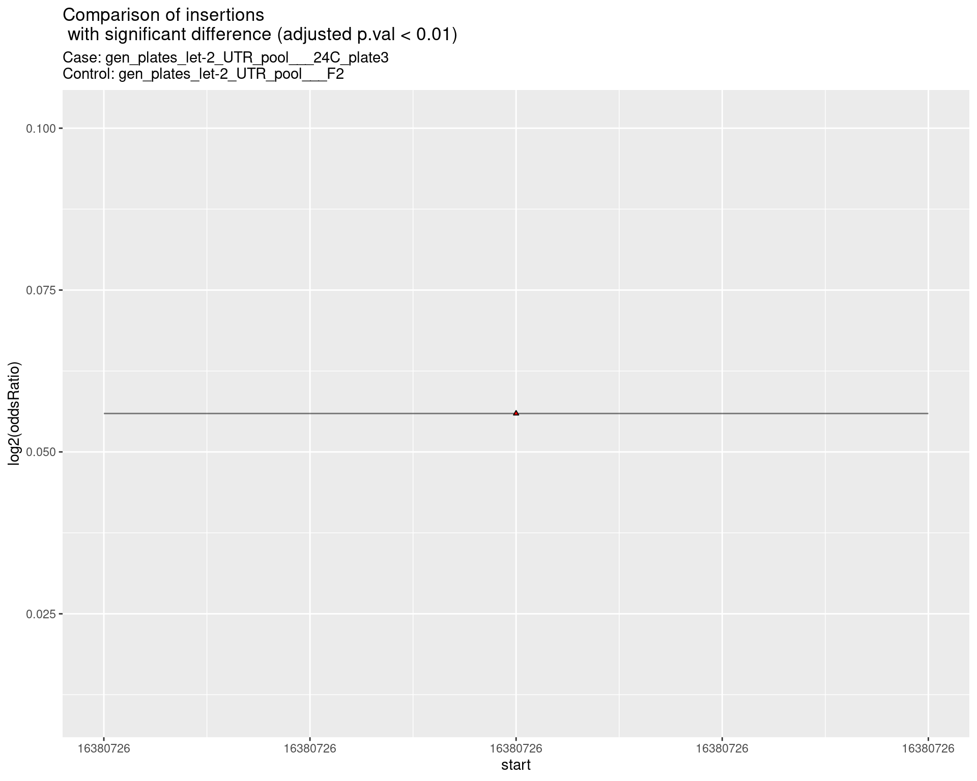
2.2.2 Comparison: gen_plates_let-2_UTR_pool_24C_plate3_vs_gen_plates_let-2_UTR_pool_F2 {.tabset .tabset-pills .tabset-fade}
2.2.2.1 segment_plot
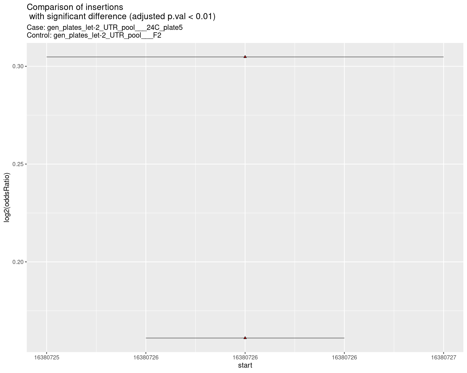
2.2.3 Comparison: gen_plates_let-2_UTR_pool_24C_plate5_vs_gen_plates_let-2_UTR_pool_F2 {.tabset .tabset-pills .tabset-fade}
2.2.3.1 segment_plot
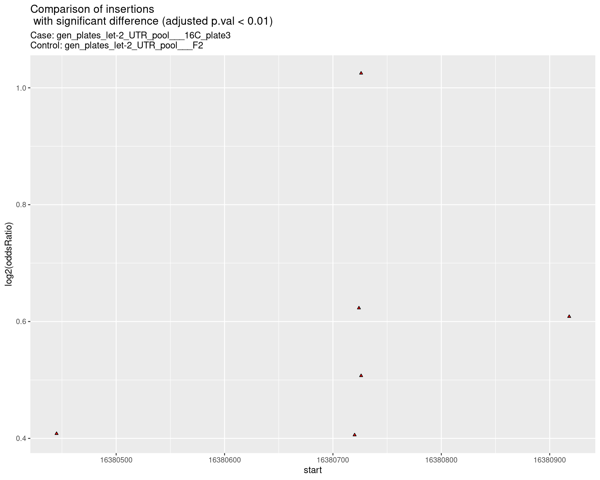
2.2.4 Comparison: gen_plates_let-2_UTR_pool_16C_plate3_vs_gen_plates_let-2_UTR_pool_F2 {.tabset .tabset-pills .tabset-fade}
2.2.4.1 segment_plot
2.2.5 Comparison: gen_plates_let-2_UTR_pool_16C_plate5_vs_gen_plates_let-2_UTR_pool_F2 {.tabset .tabset-pills .tabset-fade}
2.2.5.1 segment_plot

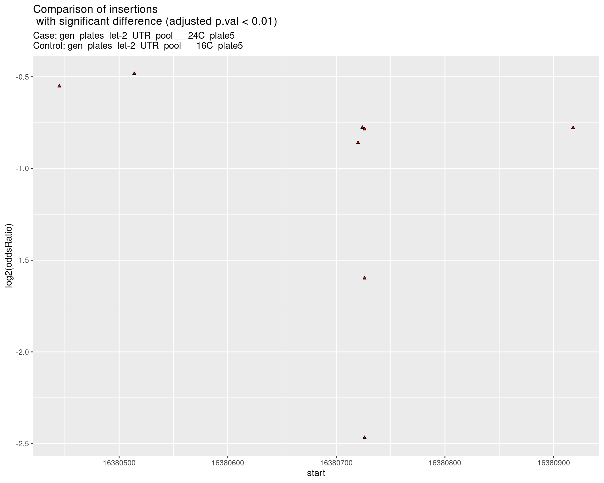
2.2.6 Comparison: gen_plates_let-2_UTR_pool_24C_plate5_vs_gen_plates_let-2_UTR_pool_16C_plate5 {.tabset .tabset-pills .tabset-fade}
2.2.6.1 segment_plot
2.2.7 Comparison: gen_plates_let-2_UTR_pool_24C_plate3_vs_gen_plates_let-2_UTR_pool_16C_plate3 {.tabset .tabset-pills .tabset-fade}
2.2.7.1 segment_plot